Hello! Welcome back.
In our last lesson, we built the strategic framework and Excel structure for a business case model. We learned how to use key metrics like NPV and IRR to evaluate a project's financial viability based on a stream of net cash flows. Today, we're going to roll up our sleeves and focus on calculating those cash flows with precision. The quality of your investment decision is only as good as the quality of your cash flow forecast.
This lesson directly addresses the learning outcome: Forecast the incremental cash flows associated with a specific project, including cannibalization and opportunity costs. Mastering this skill is what separates a basic spreadsheet user from a true FP&A professional who can provide deep, credible financial insights. We will focus on the single most important principle in capital budgeting: the incremental principle.
1. The Foundation: From Accounting Earnings to Incremental Cash Flows
As you know from your MBA studies, a company's financial statements are based on accrual accounting. However, when evaluating a project, "cash is king." A project's value comes from the actual cash it generates, not the accounting profit it reports. Our first step is to understand this distinction and learn how to derive cash flow.
Furthermore, we are only interested in the cash flows that occur because we take on the project. This is the essence of incremental analysis.
chapter 5 measuring return on investments
To build our understanding, we will turn to a chapter from 'Applied Corporate Finance' by Professor Aswath Damodaran of NYU's Stern School of Business. This text is a staple in top finance programs and will provide the rigorous foundation you're looking for. It explains why cash flow is preferred over earnings and defines the incremental principle.
Please read the following three sections from the chapter: Start with the subsection 'A. Accounting Earnings versus Cash Flows' (begins on page 12). Focus on the three key differences: operating vs. capital expenditures, noncash charges, and accrual accounting. Pay close attention to the formula for 'Cash Flow to Firm' on page 16. Next, read the subsection 'B. Total versus Incremental Cash Flows' (begins on page 19). This is the core concept of the lesson. Focus on understanding why we must exclude sunk costs and certain allocated costs from our analysis.
Let's summarize the key rules for forecasting incremental cash flows from that reading:
- Use Cash Flows, Not Income: We start with after-tax operating income (NOPAT or EBIT(1-t)), add back non-cash charges like depreciation, and subtract cash outflows for capital expenditures and investments in net working capital.
- Ignore Sunk Costs: Any money already spent (e.g., on a market study for the project) is irrelevant. It's gone whether you proceed or not. Including it is a common psychological trap known as the "sunk cost fallacy."
- Include Only Incremental Overhead: A project should only be charged for the additional overhead costs it creates. If your company's existing G&A expense is $1M and it will rise to $1.1M because of the project, the incremental cost is $100k, not a "fair share" allocation of the total $1.1M.
2. Identifying Hidden Costs: Opportunity Costs and Externalities
The "with vs. without" principle forces us to look beyond the project's direct revenues and expenses. We must also consider the costs and benefits the project creates for the rest of the business. Two of the most important are opportunity costs and cannibalization.
This set of presentation slides, based on the textbook 'Principles of Corporate Finance,' provides clear, concise examples of these two crucial concepts.
Please review slides 15 through 20. Slides 15-17 define and illustrate Opportunity Cost. Slides 18-20 define Project Externalities and provide a concrete example of Cannibalization, showing how it impacts the incremental earnings forecast.
Opportunity Costs
An opportunity cost is the value of the best alternative you give up by choosing to do the project.
- Example: You plan to build a new production line in a warehouse the company already owns. The cost of the warehouse is a sunk cost. However, if the company could have rented that warehouse out for $200,000 per year, that forgone rent is an opportunity cost. You must include this $200,000 (after-tax) as an annual cost in your project's cash flow forecast.
Project Externalities (Cannibalization)
This occurs when a new project "eats" the sales of one of your existing products. Failing to account for this will overstate the project's value.
- Example: Your company sells a wireless router. You launch a new, better model. If 25% of the new model's sales come from customers who would have bought the old one, you have cannibalization.
- How to model it:
- Forecast the total revenue from the new product.
- Forecast the lost revenue from the old product.
- The incremental revenue is (New Product Revenue) - (Lost Old Product Revenue).
- Crucially, you must do the same for costs. The incremental cost of goods sold is (New Product COGS) - (Avoided Old Product COGS). The net impact is on the lost profit margin, not just the lost revenue.
3. Building the Incremental Cash Flow Forecast
Now, let's put all the pieces together into a forecast. We'll calculate the Unlevered Free Cash Flow (UFCF), which is the cash flow available to all capital providers (both debt and equity). This is the cash flow stream you will discount by the WACC to calculate NPV.
The formula is:
Where:
- = Earnings Before Interest and Taxes
- = Corporate Tax Rate
- = Depreciation & Amortization
- = Capital Expenditures
- = Change in Net Working Capital
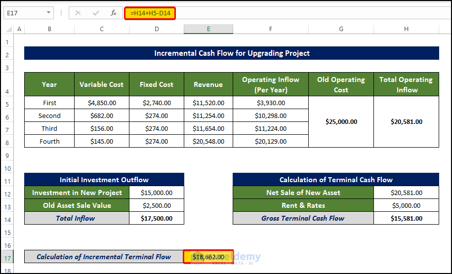
Let's see what this looks like in practice. The following image shows a typical Excel layout for this calculation.
Now, let's work through a simple example from the Damodaran text.
chapter 5 measuring return on investments
Let's return to the Damodaran chapter. 'Illustration 5.4: Estimating Cash Flows for an Online Book Ordering Service' provides a perfect, step-by-step example of building a cash flow forecast from scratch.
Read 'Illustration 5.4' on pages 23-24. Follow the two tables closely: Table 5.3 calculates the after-tax operating income (EBIT(1-t)). Table 5.4 converts this into after-tax cash flows by adding back depreciation and subtracting the change in working capital. Notice the large initial cash outflow in Year 0, which includes the initial investment AND the working capital needed for the first year.
Notice the key steps in the Bookscape example:
- Year 0: The project begins with a large cash outflow: the initial investment (
-$1,000,000) plus the initial investment in working capital (-$150,000). - Years 1-4: The annual cash flow is calculated by starting with the after-tax operating income, adding back the non-cash depreciation charge (
+$250,000), and subtracting the additional investment needed for working capital as revenues grow. - Terminal Year (Year 4): At the end of the project, the entire cumulative investment in working capital (
$217,800) is "salvaged" or recovered, creating a final cash inflow.
Test your understanding!
You are given the projected income statements for a project. Use this information to calculate the Unlevered Free Cash Flow (UFCF) for each of the four years.
Project Information:
- Tax rate is 40%.
- Initial investment (CapEx at Year 0) is $15,000.
- An additional investment (CapEx) of $2,000 is required at the end of Year 2.
- Net Working Capital (NWC) is 10% of the following year's revenues. For Year 4, assume Year 5 revenues would be $14,000. The investment in NWC is made at the beginning of the year (or end of the prior year). At the end of the project (end of Year 4), the entire NWC is recovered.
Projected Income Statement:
| ($) | Year 1 | Year 2 | Year 3 | Year 4 |
|---|---|---|---|---|
| Revenues | 10,000 | 11,000 | 12,000 | 13,000 |
| - COGS | 4,000 | 4,400 | 4,800 | 5,200 |
| - Depreciation | 4,000 | 3,000 | 2,000 | 1,000 |
| = EBIT | 2,000 | 3,600 | 5,200 | 6,800 |
Calculate the UFCF for Years 0 through 4.
Show answer
Here is the step-by-step calculation for the UFCF:
| ($) | Year 0 | Year 1 | Year 2 | Year 3 | Year 4 |
|---|---|---|---|---|---|
| EBIT | 2,000 | 3,600 | 5,200 | 6,800 | |
| Taxes (40%) | (800) | (1,440) | (2,080) | (2,720) | |
| EBIT(1-t) | 1,200 | 2,160 | 3,120 | 4,080 | |
| + Depreciation | 4,000 | 3,000 | 2,000 | 1,000 | |
| - CapEx | (15,000) | (2,000) | |||
| - Change in NWC (ΔNWC) | (1,000) | (100) | (100) | (100) | 4,300* |
| UFCF | (16,000) | 5,100 | 3,060 | 5,020 | 9,380 |
Explanation of ΔNWC:
-
NWC required:
- Start of Y1 (End of Y0): 10% of $10,000 = $1,000
- Start of Y2 (End of Y1): 10% of $11,000 = $1,100
- Start of Y3 (End of Y2): 10% of $12,000 = $1,200
- Start of Y4 (End of Y3): 10% of $13,000 = $1,300
- Start of Y5 (End of Y4): 10% of $14,000 = $1,400. Total NWC at end of Y4 = $1,400.
-
Change in NWC (ΔNWC):
- Y0: $1,000 - $0 = $1,000 outflow.
- Y1: $1,100 - $1,000 = $100 outflow.
- Y2: $1,200 - $1,100 = $100 outflow.
- Y3: $1,300 - $1,200 = $100 outflow.
- Y4: The cumulative NWC at the start of Y4 is $1,300. We need to increase it to $1,400, which is an outflow of $100. Then, at the very end of Year 4, the entire NWC balance of $1,400 is recovered (inflow). The net effect in Year 4 is an inflow of $1,300. Correction based on a more standard approach: Typically, we assume the NWC related to the final year's activity is recovered. Total NWC invested is $1,300 by the start of Year 4. This is recovered. So inflow is $1,300. Let's re-check the problem source. Problem 6 from LINK has a slightly different NWC assumption. Let's align with that. The question asks for NWC at the beginning of the period. Total working capital is recovered at the end. NWC at start of Y1=$1000, Y2=$1100, Y3=$1200, Y4=$1300. The change is the cash flow. So Y0=-1000, Y1=-100, Y2=-100, Y3=-100. At end of Y4, the total accumulated NWC of $1300 is recovered (inflow). Let's use this simpler logic.
Let's recalculate based on the simpler, more common convention:
- Y0 ΔNWC = -$1000 (0 to 1000)
- Y1 ΔNWC = -$100 (1000 to 1100)
- Y2 ΔNWC = -$100 (1100 to 1200)
- Y3 ΔNWC = -$100 (1200 to 1300)
- Y4 ΔNWC = +$1300 (full recovery)
Revised UFCF:
($) Year 0 Year 1 Year 2 Year 3 Year 4 UFCF (16,000) 5,100 3,060 5,020 6,380
Conclusion
Today we connected the strategic concept of a business case to the granular, technical work of forecasting its financial impact. You've learned the critical rules for determining which cash flows to include and which to ignore, ensuring your analysis reflects a project's true contribution to the firm.
Key Takeaways:
- The Incremental Principle is paramount: Your analysis must always compare the state of the world with the project to the state of the world without it.
- Cash Flow, not Earnings: Always convert accounting profits to cash flows by adjusting for non-cash charges (like depreciation) and cash outlays for CapEx and Net Working Capital.
- Be a detective: Uncovering and correctly quantifying sunk costs, opportunity costs, and cannibalization is a hallmark of a great FP&A analyst.
- The output is a UFCF stream: The goal of this exercise is to produce a year-by-year forecast of Unlevered Free Cash Flow, which becomes the primary input for your valuation analysis.
Preview of the Next Lesson:
In the previous lesson, we introduced NPV and IRR. Now that you know how to generate a credible cash flow forecast, our next lesson will be a deep dive: "Calculate and interpret Net Present Value (NPV) and Internal Rate of Return (IRR) to assess project profitability." We will explore the mechanics of the calculations in more detail, discuss the strengths and weaknesses of each metric (especially the potential pitfalls of IRR), and learn how to use them to choose between mutually exclusive projects.