Optimal Consumption: Tangency Condition

The Optimal Choice: Where Willingness Meets Affordability

A rational consumer aims to reach the highest possible indifference curve, as higher curves correspond to greater utility. However, their choice is constrained by their budget. The optimal bundle, therefore, must satisfy two conditions:

1. It must be affordable, meaning it lies on the budget line.
2. It must be the most preferred among all affordable bundles.

Let's visualize this.

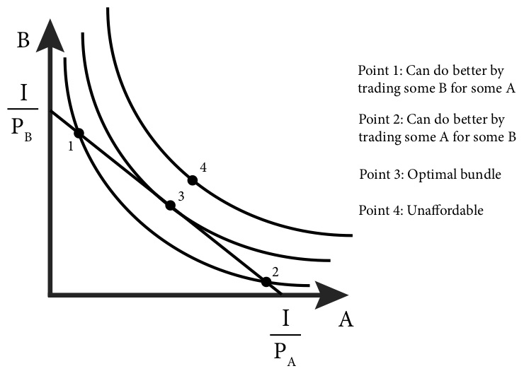
As the image illustrates, the optimal point is where the budget line just touches, or is tangent to, an indifference curve. At any other point on the budget line (like Points 1 or 2), the indifference curve crosses the budget line, implying that the consumer can move along the budget line to reach a higher, more preferred indifference curve.

This tangency has a crucial mathematical implication. At the point of optimal choice, the slope of the indifference curve must equal the slope of the budget line.

This leads to the core condition for an interior optimum:

This simplifies to the celebrated tangency condition:

This equation provides a powerful economic intuition: the consumer adjusts their consumption until the rate at which they are willing to trade one good for another (the MRS) is exactly equal to the rate at which the market allows them to trade (the price ratio). If $MRS>P_X/P_Y$, the consumer values an extra unit of X more than the market does, so they will buy more X and less Y. This continues until the diminishing MRS brings the ratio back to equality.

The following reading explains this concept clearly.

Solving for the Optimal Bundle

To find the optimal quantities of X and Y, you need to solve a system of two equations with two unknowns ($X$ and $Y$):

1. The Tangency Condition: $\frac{M{U}_X}{M{U}_Y}=\frac{P_X}{P_Y}$
2. The Budget Constraint: $P_{X}X+P_{Y}Y=I$

The first equation ensures the consumer is at a point of tangency, maximizing utility for a given level of expenditure. The second equation ensures this point is actually affordable and that the entire budget is spent (which we assume, given "more is better").

The following video provides a clear, step-by-step example of how to apply this method.

A More Formal Approach: The Lagrangian Method

Given your background in statistics and quantitative methods, you might appreciate a more formal and powerful technique for solving this type of constrained optimization problem: the Lagrange multiplier method. This approach is widely used in economics and other sciences.

The goal is to maximize the utility function $U(X,Y)$ subject to the constraint that $P_{X}X+P_{Y}Y=I$. We can rewrite the constraint as $I-P_{X}X-P_{Y}Y=0$.

We then form the Lagrangian function, $\mathcal{L}$, which combines the objective function and the constraint into a single expression:

Here, $\lambda$ (lambda) is the Lagrange multiplier. To find the maximum, we take the partial derivatives of $\mathcal{L}$ with respect to $X$, $Y$, and $\lambda$ and set them all to zero. These are the first-order conditions:

1. $\frac{\partial \mathcal{L}}{\partial X}=\frac{\partial U}{\partial X}-\lambda P_X=0⟹M{U}_X=\lambda P_X$
2. $\frac{\partial \mathcal{L}}{\partial Y}=\frac{\partial U}{\partial Y}-\lambda P_Y=0⟹M{U}_Y=\lambda P_Y$
3. $\frac{\partial \mathcal{L}}{\partial \lambda }=I-P_{X}X-P_{Y}Y=0$

Notice what this system gives us. The third condition is simply our budget constraint. If we rearrange the first two conditions and then divide the first by the second, we get:

This is precisely the tangency condition we started with. The Lagrangian method is a systematic way to derive the necessary conditions for an optimum.

Practice Problem

Let's work through a problem to solidify your understanding. A consumer has a utility function given by $U(X,Y)=X^{0.25}{Y}^{0.75}$. Their income is $I=\$200$, the price of good X is $P_X=\$5$, and the price of good Y is $P_Y=\$15$.

Find the optimal consumption bundle ($X^{\ast },Y^{\ast }$).

Solution:

1. Find the MRS. This is a Cobb-Douglas function, so we can use the formula from the previous lesson, $MRS=\frac{\alpha }{\beta }\frac{Y}{X}$, with $\alpha =0.25$ and $\beta =0.75$.

   $$MR{S}_{XY}=\frac{0.25}{0.75}\frac{Y}{X}=\frac{1}{3}\frac{Y}{X}$$

2. Set up the tangency condition. We set the MRS equal to the price ratio, $P_X/P_Y$.

   $$\frac{1}{3}\frac{Y}{X}=\frac{5}{15}=\frac{1}{3}$$

   Simplifying this gives our first key equation, which describes the relationship between X and Y at any tangent point:

   $$\frac{Y}{X}=1⟹Y=X$$

3. Use the budget constraint. Our second equation is the budget line:

   $$5X+15Y=200$$

4. Solve the system. Now we substitute the result from the tangency condition ($Y=X$) into the budget constraint:

   $$5X+15(X)=200$$ $$20X=200$$ $$X^{\ast }=10$$

   Since $Y=X$, we have:

   $$Y^{\ast }=10$$

The optimal consumption bundle is (10, 10). The consumer will buy 10 units of good X and 10 units of good Y to maximize their utility.

Conclusion

In this lesson, we have reached the pinnacle of basic consumer theory. By combining the budget constraint and indifference curves, we can now precisely solve for the consumption bundle that a rational individual will choose.

Key Takeaways:

• The optimal consumption bundle is located where the budget line is tangent to the highest possible indifference curve.
• This tangency corresponds to the mathematical condition that the Marginal Rate of Substitution equals the price ratio: $MR{S}_{XY}=P_X/P_Y$.
• To solve for the optimal bundle, you must solve a system of two equations: the tangency condition and the budget constraint.
• The Lagrangian method provides a more formal framework for solving constrained optimization problems and yields the same conditions.

In our next lesson, we will look at the same problem from a slightly different angle. By rearranging the tangency condition, we will derive the equi-marginal principle, which offers another powerful intuition about optimal consumer choice related to getting the best "bang for your buck."