Optimal Consumption: The Equi-Marginal Principle

The "Bang for Your Buck" Principle

The real power of the equi-marginal principle lies in its economic intuition. Let's break down the term $M{U}_X/P_X$.

• $M{U}_X$ is the marginal utility of good X: the extra satisfaction from consuming one more unit of X.
• $P_X$ is the price of good X.
• Therefore, the ratio $M{U}_X/P_X$ represents the marginal utility per dollar spent on good X. It's the "bang for your buck" you get from spending your next dollar on good X.

The principle states that to maximize utility, a consumer should allocate their budget so that the marginal utility per dollar is equal for every good they buy.

To understand why, consider what happens if this condition is not met. Suppose:

For example, let's say the marginal utility per dollar for pizza is 5 utils, while for burritos it's only 2 utils. A rational consumer would realize they could increase their total utility by reallocating their spending. By spending one dollar less on burritos, they lose 2 utils. But by spending that same dollar on pizza, they gain 5 utils, for a net gain of 3 utils. The consumer will continue to shift spending from burritos to pizza until the "bang for the buck" equalizes. As they buy more pizza, its marginal utility falls (due to diminishing marginal utility), and as they buy fewer burritos, their marginal utility rises, eventually bringing the two ratios into balance.

The following brief reading provides an excellent summary of this core idea.

Applying the Principle: The Cardinal Approach

One way to find the optimal bundle is by using a table of utility values, an approach known as cardinal utility analysis. This method involves calculating the $MU/P$ ratio for each good at different quantities and finding the combination that satisfies both the equi-marginal principle and the budget constraint.

The video below provides a comprehensive walkthrough of this numerical method, which is a common type of problem in economics exams.

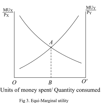
The process shown in the video can be visualized by plotting the $MU/P$ curves for each good against the quantity consumed (or money spent). The optimal allocation is found at the intersection of these two curves, as this is the point where the marginal utility per dollar is equalized.

The Formal Derivation and the Meaning of $\lambda$

Your background in quantitative methods will appreciate seeing how the equi-marginal principle emerges directly from the Lagrangian method we discussed in the last lesson. Recall the first-order conditions from setting up the utility maximization problem:

1. $M{U}_X-\lambda P_X=0⟹M{U}_X=\lambda P_X$
2. $M{U}_Y-\lambda P_Y=0⟹M{U}_Y=\lambda P_Y$

By simply rearranging these two equations, we get:

This immediately leads to our principle:

This more formal derivation also reveals the economic meaning of the Lagrange multiplier, $\lambda$. It represents the marginal utility of income—the "bang" you get from the last dollar in your budget. At the optimum, the marginal utility per dollar spent on any good is equal to this value.

The following reading from MIT OpenCourseWare formalizes this derivation and the interpretation of $\lambda$.

Practice Problem

Let's solve for an optimal bundle using the equi-marginal principle directly. A consumer has the utility function $U(X,Y)=X^{1/3}{Y}^{2/3}$. Their income is $I=\$600$, the price of good X is $P_X=\$10$, and the price of good Y is $P_Y=\$20$.

Find the optimal consumption bundle ($X^{\ast },Y^{\ast }$).

Solution:

1. Find the Marginal Utilities. We take the partial derivatives of the utility function:

   $$M{U}_X=\frac{\partial U}{\partial X}=\frac{1}{3}{X}^{-2/3}{Y}^{2/3}$$ $$M{U}_Y=\frac{\partial U}{\partial Y}=\frac{2}{3}{X}^{1/3}{Y}^{-1/3}$$

2. Set up the Equi-marginal Condition. We set up the $M{U}_X/P_X=M{U}_Y/P_Y$ equation:

   $$\frac{\frac{1}{3}{X}^{-2/3}{Y}^{2/3}}{10}=\frac{\frac{2}{3}{X}^{1/3}{Y}^{-1/3}}{20}$$

3. Solve for Y in terms of X. Now, we simplify the expression.

   $$\frac{1}{30}{X}^{-2/3}{Y}^{2/3}=\frac{2}{60}{X}^{1/3}{Y}^{-1/3}$$ $$\frac{1}{30}{X}^{-2/3}{Y}^{2/3}=\frac{1}{30}{X}^{1/3}{Y}^{-1/3}$$

   The $\frac{1}{30}$ terms cancel out. To simplify the exponents, multiply both sides by $X^{2/3}{Y}^{1/3}$:

   $$Y^{2/3}\cdot Y^{1/3}=X^{1/3}\cdot X^{2/3}$$ $$Y^1=X^1⟹Y=X$$

   This gives us the relationship between X and Y at the optimal bundle.

4. Use the Budget Constraint. Substitute $Y=X$ into the budget constraint $10X+20Y=600$:

   $$10X+20(X)=600$$ $$30X=600$$ $$X^{\ast }=20$$

   Since $Y=X$, we have:

   $$Y^{\ast }=20$$

The optimal consumption bundle is (20, 20). The consumer maximizes their utility by purchasing 20 units of good X and 20 units of good Y.

Conclusion

In this lesson, we reframed the consumer's optimization problem through the lens of the equi-marginal principle. This perspective provides a powerful and practical intuition for utility maximization: a rational consumer allocates their spending to equalize the "bang for the buck" from the last dollar spent on every good.

Key Takeaways:

• The optimal consumption bundle is found where the marginal utility per dollar spent is equal across all goods: $M{U}_X/P_X=M{U}_Y/P_Y$.
• This principle is an algebraic rearrangement of the tangency condition ($MRS=P_X/P_Y$) and thus represents the same underlying economic logic.
• If $M{U}_X/P_X>M{U}_Y/P_Y$, a consumer can increase total utility by shifting spending from good Y to good X.
• The common value of the $MU/P$ ratios at the optimum is equal to $\lambda$, the marginal utility of income.

In our next lesson, we will continue to build on this framework by analyzing how the optimal consumption bundle changes when a consumer's income rises or falls.