Indifference Curves and the Marginal Rate of Substitution

From Utility to Indifference Curves

Recall that a utility function, $U(X,Y)$, assigns a numerical value of satisfaction to any given bundle of goods $(X,Y)$. An indifference curve is essentially a contour map of this function. It connects all the consumption bundles that provide the consumer with the exact same level of utility. Just as contours on a topographical map connect points of equal elevation, an indifference curve connects bundles of equal satisfaction.

To construct one, we can start with an indifference schedule—a table of combinations of goods that yield the same utility.

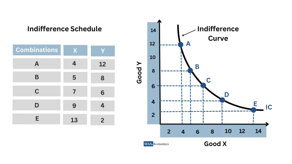
As you can see, to get more of Good X (moving from A to B), the consumer must give up some of Good Y to remain equally satisfied. This trade-off is fundamental. For most goods, indifference curves share several key properties:

1. Downward Sloping: Because we assume "more is better" (positive marginal utility for both goods), if the quantity of one good increases, the quantity of the other must decrease to keep total utility constant.
2. Higher Curves Represent Higher Utility: A bundle on a curve further from the origin contains more of at least one good, and is therefore preferred.
3. Indifference Curves Do Not Cross: This would violate the assumption of transitivity in preferences. If they crossed, the intersection point would imply two different utility levels are equal, which is a contradiction.
4. Convex to the Origin: This is the most interesting property. The curve is "bowed inward." This shape reflects a diminishing marginal rate of substitution, a concept we will now explore in detail.

The Slope: Marginal Rate of Substitution (MRS)

The slope of the indifference curve tells us the rate at which a consumer is willing to substitute one good for the other. The absolute value of this slope is called the Marginal Rate of Substitution (MRS).

For small changes, the MRS of X for Y is defined as:

It measures how many units of good Y the consumer is willing to give up to obtain one more unit of good X, while staying on the same indifference curve.

Let's look at a numerical calculation between discrete points.

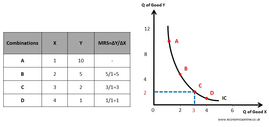
Notice that as we move down the curve from A to D, the MRS decreases from 5 to 1. This is the property of diminishing MRS. When the consumer has a lot of Y and very little X (at point A), they are willing to give up a large amount of Y (5 units) to get one more unit of X. When they have little Y and a lot of X (at point C), they are only willing to give up a small amount of Y (1 unit) to get one more unit of X. This intuition—that people prefer variety and are less willing to trade away a good that has become scarce in their bundle—is what gives indifference curves their characteristic convex shape.

The following video provides a clear definition of MRS and its relationship to the shape of the indifference curve.

A Rigorous Derivation of MRS

Your background in quantitative methods will make the formal derivation of the MRS particularly straightforward. We can express the MRS as a ratio of marginal utilities using partial derivatives.

Consider a consumer moving along an indifference curve. The total utility $U(X,Y)$ is constant. The total differential of the utility function is:

Here, $\frac{\partial U}{\partial X}$ is the marginal utility of X ($M{U}_X$), and $\frac{\partial U}{\partial Y}$ is the marginal utility of Y ($M{U}_Y$).

Since utility is constant along an indifference curve, the total change in utility, $dU$, must be zero.

Rearranging this equation to find the slope of the curve, $\frac{dY}{dX}$, gives:

The MRS is the absolute value of this slope. Therefore, we arrive at the central relationship:

The rate at which a consumer is willing to trade Y for X is equal to the ratio of the marginal utility of X to the marginal utility of Y. This makes intuitive sense: if an extra unit of X gives you twice as much utility as an extra unit of Y ($M{U}_X/M{U}_Y=2$), you should be willing to give up 2 units of Y to get 1 unit of X.

The following reading provides a concise and elegant presentation of this derivation.

Application: The Cobb-Douglas Utility Function

Let's apply this to a common and important type of utility function used in economic modeling: the Cobb-Douglas function, $U(X,Y)=A{X}^{\alpha }{Y}^{\beta }$, where A, $\alpha$, and $\beta$ are positive constants. This form is often used in CB2 exam questions.

We can find the MRS by calculating the marginal utilities first.

1. Find the Marginal Utility of X ($M{U}_X$): $$M{U}_X=\frac{\partial U}{\partial X}=A(\alpha X^{\alpha -1})Y^{\beta }$$
2. Find the Marginal Utility of Y ($M{U}_Y$): $$M{U}_Y=\frac{\partial U}{\partial Y}=A{X}^{\alpha }(\beta Y^{\beta -1})$$
3. Find the MRS: $$MR{S}_{XY}=\frac{M{U}_X}{M{U}_Y}=\frac{A\alpha X^{\alpha -1}{Y}^{\beta }}{A\beta X^{\alpha }{Y}^{\beta -1}}$$ Simplifying this expression gives: $$MR{S}_{XY}=\frac{\alpha }{\beta }\frac{Y}{X}$$

This result is powerful. It shows that for a Cobb-Douglas function, the MRS depends on the preference parameters ($\alpha$ and $\beta$) and the ratio of the quantities of the goods consumed ($Y/X$).

The following resource provides several worked examples of finding the MRS for different utility functions, including a rigorous look at the Cobb-Douglas case.

Practice Problem

Let's put your skills to the test. A consumer's preferences are represented by the utility function $U(X,Y)=X^{0.5}{Y}^{0.5}$.

1. Find the general expression for the $MR{S}_{XY}$.
2. Calculate the MRS at the consumption bundle (X=4, Y=16).
3. Interpret the value you found in part 2.

Solution:

1. This is a Cobb-Douglas function with $\alpha =0.5$ and $\beta =0.5$. Using our formula $MRS=\frac{\alpha }{\beta }\frac{Y}{X}$:

   $$MR{S}_{XY}=\frac{0.5}{0.5}\frac{Y}{X}=\frac{Y}{X}$$

   Alternatively, by first principles:
   $M{U}_X=0.5X^{-0.5}{Y}^{0.5}$
   $M{U}_Y=0.5X^{0.5}{Y}^{-0.5}$
   $MR{S}_{XY}=\frac{0.5X^{-0.5}{Y}^{0.5}}{0.5X^{0.5}{Y}^{-0.5}}=\frac{Y}{X}$

2. At the bundle (X=4, Y=16):

   $$MRS=\frac{16}{4}=4$$

3. Interpretation: At this point on the indifference curve, the consumer is willing to give up 4 units of Good Y to obtain 1 additional unit of Good X and remain just as satisfied. The subjective value of one more unit of X is 4 units of Y.

Conclusion

In this lesson, we have delved into the representation of consumer preferences. You've learned how to construct indifference curves from a utility schedule and, more importantly, how to interpret their slope both intuitively and mathematically.

Key Takeaways:

• An indifference curve shows all combinations of two goods that provide a consumer with the same level of utility.
• The absolute value of the slope of an indifference curve is the Marginal Rate of Substitution (MRS). It represents the rate at which a consumer is willing to trade one good for another.
• The MRS can be calculated as the ratio of marginal utilities: $MR{S}_{XY}=\frac{M{U}_X}{M{U}_Y}$.
• For most standard preferences, indifference curves are convex due to a diminishing MRS: the more of a good you have, the less you are willing to give up of other goods to get even more of it.

We have now established the two pillars of consumer theory: the budget line (what the consumer can do) and the indifference curve (what the consumer wants to do). In the next lesson, we will combine these two concepts to find the consumer's optimal consumption bundle—the affordable point that yields the highest possible utility.