Budget Lines and Relative Prices

Introduction

In our last lesson, we explored the concept of utility, which models the satisfaction a consumer derives from consuming goods. You learned to calculate marginal utility and saw how the law of diminishing marginal utility can be expressed mathematically as a concave utility function. This gave us a framework for what a consumer wants: to maximize utility.

Now, we turn to the other crucial piece of the consumer choice puzzle: what a consumer can afford. This lesson introduces the budget constraint, the limit that income and market prices impose on consumption choices. Our objective is to construct the graphical representation of this constraint—the budget line—and to precisely interpret its slope as a ratio of relative prices. This will set the stage for combining what a consumer wants with what they can afford to determine their optimal choice.

The Budget Constraint

At its heart, the consumer's problem is about making the best choice from a limited set of options. The budget constraint defines this set of feasible options. We assume a consumer has a fixed amount of income, which we'll call $M$ , to spend on two goods, X and Y. The prices of these goods are given by the market as $P_{X}$ and $P_{Y}$ , respectively.

The total expenditure on goods X and Y is given by $P_{X} Q_{X} + P_{Y} Q_{Y}$ , where $Q_{X}$ and $Q_{Y}$ are the quantities of each good purchased. The budget constraint simply states that this total expenditure cannot exceed the consumer's income:

P_{X} Q_{X} + P_{Y} Q_{Y} \leq M

The collection of all consumption bundles $(Q_{X}, Q_{Y})$ that satisfy this inequality is called the budget set. It includes every combination of goods the consumer can afford.

To simplify our analysis, economists typically focus on the budget line, which represents the bundles that a consumer can purchase if they spend their entire income. The equation for the budget line is therefore:

P_{X} Q_{X} + P_{Y} Q_{Y} = M

This is a reasonable assumption because, as we saw in the last lesson, utility generally increases with consumption (as long as marginal utility is positive). A rational consumer aiming to maximize utility would not leave any income unspent.

Let's watch a video that introduces this concept and sets up the problem.

Chapter 21: Theory of Consumer Choice - Utility Maximization

This video, "Theory of Consumer Choice - Utility Maximization" by Dr.AzevedoEcon, provides a clear introduction to the budget constraint.

Please watch the section from the beginning, which outlines the consumer's problem and defines the budget constraint as the set of affordable goods and services, making the simplifying assumption that all income is spent.

Constructing the Budget Line

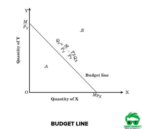
The budget line is a linear equation, which means we can graph it as a straight line. To do this, we need to find the two points where the line intersects the axes of our graph, where the axes represent the quantity of Good X and the quantity of Good Y.

Vertical Intercept (Quantity of Y): This point represents the maximum amount of Good Y the consumer can buy if they spend zero on Good X. Setting $Q_{X} = 0$ in the budget equation gives us $P_{Y} Q_{Y} = M$ , which means $Q_{Y} = M / P_{Y}$ .
Horizontal Intercept (Quantity of X): Similarly, this is the maximum amount of Good X the consumer can buy if they spend zero on Good Y. Setting $Q_{Y} = 0$ gives $P_{X} Q_{X} = M$ , so $Q_{X} = M / P_{X}$ .

The budget line is the straight line drawn between these two intercepts.

This graph illustrates a standard budget line. The vertical intercept is M/Py, the maximum quantity of Y affordable, and the horizontal intercept is M/Px, the maximum quantity of X affordable. The line itself shows all combinations of X and Y that exhaust the consumer's income, M. The area labeled 'A' is the affordable set (budget set), while point 'B' is unaffordable.

Let's see how this works with a numerical example.

Chapter 21: Theory of Consumer Choice - Utility Maximization

We'll continue with the same video, which now walks through a concrete example.

Watch the segment from the numerical example, where the presenter uses an income of $500 and prices for pizzas and Cokes to calculate different affordable bundles. Then continue from graphing the constraint, where he plots the intercepts and draws the resulting budget line. Pay close attention to how the intercepts are calculated as Income / Price.

The Slope of the Budget Line: The Relative Price Ratio

The slope of the budget line is one of its most important features. It tells us the rate at which the market permits the consumer to trade one good for the other. As a statistician familiar with linear models, you'll recognize that we can find the slope by rearranging the budget line equation into the standard slope-intercept form, $y = m x + c$ .

Let's solve the budget equation for $Q_{Y}$ , the variable on our vertical axis:

P_{X} Q_{X} + P_{Y} Q_{Y} = M

P_{Y} Q_{Y} = M - P_{X} Q_{X}

Q_{Y} = \frac{M}{P _{Y}} - \frac{P _{X}}{P _{Y}} Q_{X}

From this form, we can see two things:

The vertical intercept is indeed $M / P_{Y}$ , as we determined earlier.
The slope of the budget line is $- \frac{P _{X}}{P _{Y}}$ .

The negative sign shows that the line is downward sloping, which makes intuitive sense: to get more of one good, you must give up some of the other. The magnitude of the slope, $\frac{P _{X}}{P _{Y}}$ , is known as the relative price ratio.

This ratio represents the opportunity cost of consuming one more unit of Good X, measured in units of Good Y. For example, if a pizza ( $P_{X}$ ) costs $10 and a Coke ( $P_{Y}$ ) costs $2, the relative price ratio is $10/2 = 5$ . This means the opportunity cost of one more pizza is 5 Cokes. To free up the $10 needed to buy a pizza, a consumer must forgo purchasing 5 Cokes.

The following resources provide a focused look at this algebraic derivation and interpretation.

Understanding Slopes of Budget Lines (Budget Constraint)

The video "Understanding Slopes of Budget Lines" from Economicsfun provides a concise, step-by-step algebraic derivation.

Watch from the beginning of the derivation to see the budget equation transformed into the slope-intercept form. Then, continue to the next part on interpreting the slope as the ratio of prices.

For a more formal written explanation, you can refer to the following text.

Chapter 6: Consumer's Decision 1 Budget constraint 2 A ...

This PDF from the University of Western Ontario offers a rigorous definition of the budget constraint and slope.

Read the section titled "Budget constraint". Focus on the final paragraph, which interprets the slope −p_1/p_2 as the "rate of exchange" between the two goods, reinforcing the idea of opportunity cost.

How the Budget Line Changes

Understanding how the budget line responds to changes in income and prices is essential.

Changes in Income (M): If a consumer's income changes while prices remain constant, the budget line will shift.
- An increase in income shifts the budget line outward, parallel to the original. The consumer can now afford more of both goods. The slope remains the same because the relative price ratio $(P_{X} / P_{Y})$ has not changed.
- A decrease in income shifts the budget line inward, parallel to the original.
Changes in Prices ( $P_{X}$ or $P_{Y}$ ): If the price of one good changes, the budget line will pivot.
- If the price of Good X ( $P_{X}$ ) falls, the horizontal intercept ( $M / P_{X}$ ) moves to the right, but the vertical intercept ( $M / P_{Y}$ ) remains fixed. The budget line pivots outward, becoming flatter. The consumer can now buy more of Good X, and the opportunity cost of Good X has decreased.
- If the price of Good X rises, the budget line pivots inward, becoming steeper.

The following video segments provide an excellent visual summary of these effects.

Chapter 21: Theory of Consumer Choice - Utility Maximization

Let's return to Dr.AzevedoEcon's video for a final time to see these dynamics in action.

First, watch the demonstration of an income change, which shows the parallel shift. Then, observe how a price change for one good causes the budget line to pivot. Finally, the video provides a quick visual summary of the four possible price pivots.

Practice Problem

Let's apply these concepts. The CB2 exam often includes questions requiring you to construct and interpret budget lines. Consider this scenario, adapted from a past exam paper:

A consumer has an income of £600. They can spend it on Good X, which costs £20 per unit, or Good Y, which costs £40 per unit.

Write the equation for this consumer's budget line.
Calculate the vertical and horizontal intercepts.
Calculate and interpret the slope of the budget line.

Solution:

Equation: The budget line is $20 Q_{X} + 40 Q_{Y} = 600$ .
Intercepts:
- Horizontal intercept ( $Q_{Y} = 0$ ): $20 Q_{X} = 600 ⟹ Q_{X} = 30$ .
- Vertical intercept ( $Q_{X} = 0$ ): $40 Q_{Y} = 600 ⟹ Q_{Y} = 15$ .
Slope:
- The slope is $- \frac{P _{X}}{P _{Y}} = - \frac{20}{40} = - 0.5$ .
- Interpretation: The opportunity cost of consuming one additional unit of Good X is 0.5 units of Good Y. To buy one more unit of X, the consumer must give up half a unit of Y.

Conclusion

In this lesson, we have constructed the budget line, which represents the frontier of a consumer's affordable consumption bundles. You now know how to build this line from income and price data and, most importantly, how to interpret its key features.

Key Takeaways:

The budget line is given by the equation $P_{X} Q_{X} + P_{Y} Q_{Y} = M$ .
The intercepts of the budget line are $M / P_{Y}$ (on the Y-axis) and $M / P_{X}$ (on the X-axis), representing the maximum quantity of each good that can be purchased.
The slope of the budget line is $- \frac{P _{X}}{P _{Y}}$ , the negative of the relative price ratio.
This slope represents the opportunity cost of one good in terms of the other—the rate at which the market allows a consumer to trade them.
Changes in income cause a parallel shift of the budget line, while changes in a single price cause a pivot.

We have now defined both the consumer's desires (utility) and their limitations (budget constraint). The next step is to bring these two concepts together. In the following lesson, we will introduce indifference curves, which graphically represent a consumer's preferences. By finding where an indifference curve is tangent to the budget line, we can solve for the consumer's optimal choice.

Recommended resources

Introduction

The Budget Constraint

Constructing the Budget Line

The Slope of the Budget Line: The Relative Price Ratio

How the Budget Line Changes

Practice Problem

Conclusion