Probability and Quantile Calculations

Introduction

In our last lesson, we constructed the logical framework for hypothesis testing, establishing the roles of the null hypothesis, p-values, and significance levels. We concluded that the p-value—the probability of observing our data, or something more extreme, if the null hypothesis is true—is the key piece of evidence we generate from a statistical test.

This lesson takes the next crucial step: learning how to calculate these probabilities using R. We will focus on two of the most important probability distributions in statistics: the Normal distribution and the Student's t-distribution. You will learn to use R's built-in functions to find probabilities (like p-values) from test statistics and to find the critical values that define rejection regions for a given significance level. Mastering these functions provides you with the foundational computational skills for nearly all the statistical tests you will perform in your research career.

From Theory to Practice: Probability Distributions in R

Probability distributions are mathematical functions that provide the probabilities of occurrence of different possible outcomes in an experiment. In R, there is a consistent naming convention for the functions that work with these distributions, typically using a one-letter prefix followed by the distribution's name (e.g., norm for normal, t for t-distribution).

The four main prefixes are:

d for the density function (the height of the probability distribution curve at a given point).
p for the probability function (the cumulative probability up to a given point, i.e., the area under the curve). This is what we use for p-values.
q for the quantile function (the inverse of the p function; gives the value corresponding to a given cumulative probability). This is what we use to find critical values.
r for random number generation from that distribution.

Today, we will focus on the d, p, and q functions for the Normal and t-distributions.

The Normal Distribution

The Normal distribution is a cornerstone of statistics, often used to model continuous variables like IQ scores, height, or blood pressure. It is defined by two parameters: its mean ( $μ$ ), which determines the center of the peak, and its standard deviation ( $σ$ ), which determines the spread of the curve.

The resource "Revisiting Probability Distributions" provides an excellent, hands-on walkthrough of the R functions for the normal distribution. We will work through its key sections.

Lab 4 Revisiting Probability Distributions | Level 2 Research Methods and Statistics Practical Skills

This guide will introduce you to the dnorm, pnorm, and qnorm functions using clear examples and visualizations. Working through it will build your practical R skills for handling continuous probability data.

First, read the brief recap to refresh your understanding of its properties. Next, we'll explore the core functions. Start with the section on R's functions for the normal distribution, which introduces the d/p/q naming pattern. Continue to the section on the density function, dnorm(). This part is important for understanding how to plot the distribution and what the "density" value means. Now for the most important function for hypothesis testing: the cumulative probability function. Read the entire section on pnorm() carefully. Pay close attention to the lower.tail argument, which is essential for calculating p-values correctly. Finally, read the section on the inverse function, the quantile function, qnorm(). This explains how to find a cutoff value (like a critical value for a test) given a certain probability.

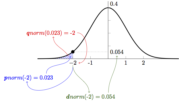
Let's consolidate what you've just read. The pnorm() function calculates the area under the curve to the left of a specified value (a quantile). This area represents the probability of getting a result less than or equal to that value. The qnorm() function does the reverse: you provide a probability (an area), and it returns the corresponding quantile.

This short video provides a great visual summary and reinforces these concepts using the IQ score example.

How to use the 4 different norm() functions in R

This video from The Data Digest will help you visualize the relationship between pnorm and qnorm.

Watch the initial IQ example to see a quick overview. Then, focus on the detailed explanations of pnorm and qnorm.

The image below, from the University of Luxembourg, provides a perfect graphical summary of how these functions relate to the standard normal distribution (a special case where $μ = 0$ and $σ = 1$ ).

This diagram illustrates the core R functions for a standard normal distribution. `dnorm(-2)` gives the height of the curve at x=-2. `pnorm(-2)` gives the cumulative area to the left of x=-2. `qnorm(0.023)` gives the x-value (-2) that corresponds to a cumulative area of 0.023.

A note on terminology: the quantile function you saw in the PharmaSUG paper (quantile(x, probs = ...)), is used to get quantiles from your actual data. The qnorm() function gets theoretical quantiles from a perfect normal distribution. This is a crucial distinction between descriptive statistics (describing your sample) and inferential statistics (comparing your sample to a theoretical model).

The Student's t-Distribution

In the real world of research, we almost never know the true population standard deviation ( $σ$ ). We have to estimate it using the standard deviation of our sample. This introduces extra uncertainty. To account for this, we use the t-distribution instead of the normal distribution, especially when our sample size is small.

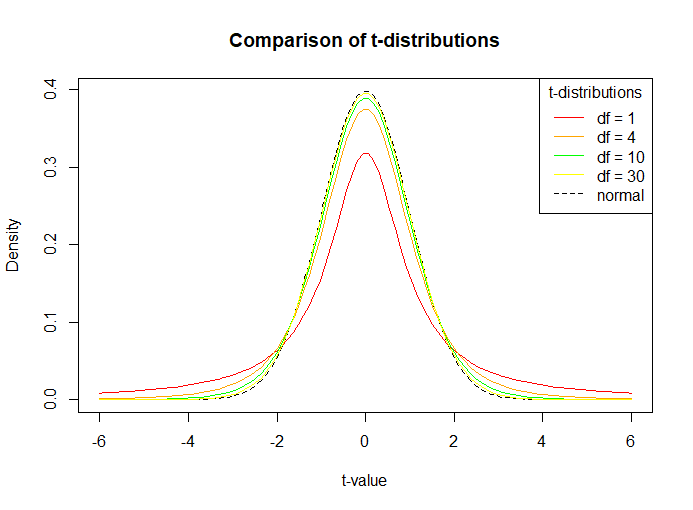
The t-distribution looks very similar to the normal distribution—it's bell-shaped and centered at zero—but it has "fatter" tails. These fatter tails mean that more extreme values are more likely, which reflects the added uncertainty from having estimated the standard deviation.

The exact shape of the t-distribution depends on a parameter called the degrees of freedom (df), which is directly related to your sample size (for many tests, df = n - 1). As the degrees of freedom increase (i.e., as your sample size gets larger), the t-distribution becomes indistinguishable from the normal distribution. This is because a larger sample gives you a more reliable estimate of the standard deviation, reducing the extra uncertainty.

This plot shows how the t-distribution (colored lines) changes with different degrees of freedom (df). Notice that as df increases from 1 to 30, the tails get thinner and the peak gets higher, approaching the shape of the standard normal distribution (dashed line).

The R functions for the t-distribution follow the same pattern as the normal distribution: dt(), pt(), and qt(). The key difference is that you must also supply the degrees of freedom (df).

The following video is an excellent tutorial on using these functions in the exact context of hypothesis testing.

t Distribution and t Scores in R | R Tutorial 3.4 | MarinStatsLectures

This MarinStatsLectures video will show you how to use pt() and qt() to calculate p-values and critical values for a t-test.

Watch from the beginning to the end. The video clearly demonstrates how to: Use pt() to find a one-sided p-value (lower.tail = FALSE). Calculate a two-sided p-value by doubling the one-sided p-value. Use qt() to find the critical t-value needed to construct a confidence interval.

Example Calculation

Let's apply this. Imagine you are conducting a small pilot study for a new medication (n=20 participants). You want to see if it changes blood pressure. After your experiment, you calculate a t-statistic of t = 2.5. Your degrees of freedom would be df = n - 1 = 19.

To find the two-sided p-value (the probability of getting a t-statistic as extreme as 2.5 or -2.5), you would calculate the area in the upper tail and double it:

pt(2.5, df = 19, lower.tail = FALSE) gives you the area in the upper tail.
2 * pt(2.5, df = 19, lower.tail = FALSE) gives you the two-sided p-value.

Let's try it in the R console:

> 2 * pt(2.5, df = 19, lower.tail = FALSE)
[1] 0.02158

The p-value is approximately 0.022. If your significance level ( $α$ ) was 0.05, you would reject the null hypothesis and conclude that the medication has a statistically significant effect on blood pressure.

Conclusion

In this lesson, you've bridged the gap between the theory of hypothesis testing and the practical application in R. You now have the tools to work with two of the most fundamental probability distributions in statistics.

Key Takeaways:

R uses a consistent d/p/q naming convention for its distribution functions.
The Normal distribution is a model for continuous data where the population mean and standard deviation are known. You can use pnorm() to find probabilities and qnorm() to find quantiles (values).
The t-distribution is used when the population standard deviation is unknown and estimated from the sample. It accounts for this extra uncertainty with "fatter tails."
The shape of the t-distribution is determined by the degrees of freedom (df). As df increases, the t-distribution approaches the normal distribution.
You can use pt() to calculate p-values from a t-statistic and qt() to find the critical t-values for hypothesis tests and confidence intervals.

Preview of the Next Lesson:
We have now explored the theoretical distributions that serve as our benchmark for statistical significance. In the next lesson, "Calculate and interpret descriptive statistics," we will turn our attention to our own data. You will learn how to use R to compute summary statistics like the mean, median, and standard deviation, which are the first step in understanding the characteristics of your sample before you compare it to these theoretical models.