Visual and Formal Normality Checks

Why is Assessing Normality so Important?

Statistical tests are often grouped into two families: parametric and non-parametric.

• Parametric tests (like the t-test) are powerful tools that can detect subtle effects, but their validity rests on certain assumptions about the data. The most common assumption is that the data follows a normal distribution.
• Non-parametric tests (like the Wilcoxon test, which we'll see later) are more flexible as they don't require the normality assumption. However, they can sometimes be less powerful, meaning they might miss a real effect that a parametric test would have caught.

Choosing the correct test is therefore a critical decision in your analysis pipeline. Checking for normality is the gatekeeping process that guides this choice, ensuring your conclusions are statistically sound.

The following resource provides a brief but clear introduction to why this check is necessary.

Visual Assessment: Histograms and Q-Q Plots

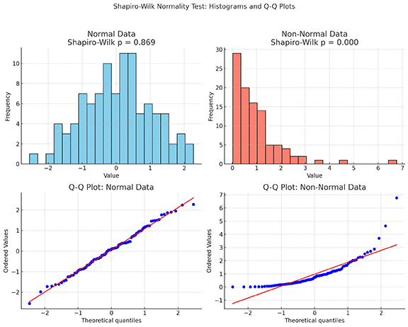
Your first step in assessing normality should always be to visualize the data. A histogram can give you a quick impression—a bell shape suggests normality—but a more precise tool is the Quantile-Quantile (Q-Q) plot.

A Q-Q plot is a scatterplot that compares the quantiles of your data (on the y-axis) against the theoretical quantiles from a perfect normal distribution (on the x-axis).

• If your data is normally distributed, the points on the plot will fall closely along a straight diagonal line.
• If your data is not normally distributed, the points will deviate from the line in a systematic pattern. For instance, a curved "U" or "S" shape can indicate that your data is skewed or has "heavy" or "light" tails compared to a normal distribution.

The image below provides a perfect illustration, contrasting a normally distributed sample with a non-normal (specifically, right-skewed) one. Notice how the points in the normal Q-Q plot hug the red line, while the points in the non-normal plot curve away from it.

To build a solid intuition for how these plots are constructed and what they represent, the following video from StatQuest is exceptionally clear.

Creating Q-Q Plots in R

You can create Q-Q plots in R using several functions. The base R qqnorm() function is simple and effective. However, for creating publication-quality graphics that align with the Tidyverse, the ggqqplot() function from the ggpubr package is an excellent choice.

The practical guide below demonstrates how to use ggqqplot() and other visualization methods.

Formal Testing: The Shapiro-Wilk Test

While visual inspection is essential, it can be subjective. To complement our plots, we use a formal statistical test. The Shapiro-Wilk test is one of the most common and reliable tests for normality.

Like other hypothesis tests, it has a null and an alternative hypothesis:

• Null Hypothesis ($H_0$): The data was sampled from a normal distribution.
• Alternative Hypothesis ($H_a$): The data was not sampled from a normal distribution.

The test produces a p-value, which you interpret as follows (typically using a significance level, $\alpha$, of 0.05):

• If $p>0.05$: You fail to reject the null hypothesis. There isn't enough evidence to say the data is non-normal.
• If $p\le 0.05$: You reject the null hypothesis. The data deviates significantly from a normal distribution.

This video explains the logic of normality tests and the interpretation of the p-value very clearly.

Running the Shapiro-Wilk Test in R

You can run the test in R using the base function shapiro.test(). Alternatively, the rstatix package (part of the tidyr ecosystem) provides a shapiro_test() function that works nicely within a %>% pipeline.

The "Statistical Analysis of Biological Data" guide demonstrates this tidy approach.

A Balanced Approach: Combining Plots and Tests

It might seem that you can just rely on the p-value from the Shapiro-Wilk test, but this is a common pitfall. The performance of normality tests is heavily influenced by sample size.

• With small samples (e.g., n < 30), tests have low "power." They might fail to detect non-normality even when it's present. In these cases, visual inspection with a Q-Q plot is arguably more important.
• With very large samples (e.g., n > 1000), tests have high "power." They can flag tiny, trivial deviations from perfect normality as "statistically significant," even if the data is "normal enough" for a parametric test to work well (thanks to a principle called the Central Limit Theorem).

The image below beautifully illustrates this point. It shows data from a non-normal (Gamma) distribution at different sample sizes.

This leads to the most important takeaway of this lesson: always use both visual inspection and a formal test.

Your workflow should be:

1. Plot your data: Look at a histogram and, more importantly, a Q-Q plot.
2. Run the test: Perform the Shapiro-Wilk test to get a p-value.
3. Synthesize:
   • If the plot looks good and p > 0.05, you can confidently assume normality.
   • If the plot looks bad and p ≤ 0.05, you have strong evidence of non-normality.
   • If the results conflict (e.g., a "good enough" plot but p ≤ 0.05 in a very large sample, or a "bad" plot but p > 0.05 in a very small sample), you must use your judgment, but the visual plot often provides the more practical guidance.

This combined approach prevents you from being misled by the limitations of a single method and is the hallmark of a careful data analyst.

Conclusion

In this lesson, you've added a critical diagnostic tool to your analytical skill set. You now understand why assessing normality is a prerequisite for many common statistical tests and how to perform this assessment using both visual and formal methods in R.

Key Takeaways:

• Parametric vs. Non-parametric: The assumption of normality determines whether you can use more powerful parametric tests (like t-tests) or must use more robust non-parametric alternatives.
• Q-Q Plots: This is your primary visual tool. Data is likely normal if the points fall along the diagonal line.
• Shapiro-Wilk Test: This is your formal statistical check. The null hypothesis is that the data is normal. A p-value ≤ 0.05 suggests the data is not normal.
• The Balanced Approach: Never rely on a p-value alone. Always combine the objective result of the Shapiro-Wilk test with the subjective but highly informative visual evidence from a Q-Q plot, being mindful of your sample size.

Preview of the Next Lesson:
Now that we've focused on understanding the distribution of a single variable, we'll shift our attention to exploring the relationship between two variables. In the next lesson, you will learn how to compute and interpret correlation coefficients, which measure the strength and direction of a linear association between two continuous variables.