Backdoor Adjustment for Causal Inference

Greetings, Detective. Your previous investigations into the studio rivalry have been masterful. You first unmasked a confounder (Package Type) that created the illusion of "Satin & Steel" being the superior studio. Then, you expertly sidestepped the trap of collider bias, proving that the negative correlation observed among elite models was a statistical phantom born from a flawed selection process.

You have learned when to adjust for a variable (a confounder) and when not to (a collider). This leaves one final, crucial piece of the puzzle. While stratifying the data by package type showed that "Velvet & Vellum" performed better in both the Basic and Premium tiers, it doesn't answer the ultimate question for a prospective client: "Overall, what is the true causal effect of choosing one studio over the other?"

To answer this, we need to move beyond simply identifying paradoxes and learn how to perform causal surgery. Today, we will arm you with the backdoor adjustment formula, a precise tool for calculating the causal effect of an action, like choosing a studio, by systematically neutralizing the influence of confounders.

From Association to Intervention: The `do`-operator

In statistics, we are accustomed to thinking in terms of conditional probabilities like $P (Y ∣ X)$ , which represents the probability of outcome Y given that we observe X. This is a statement about association. Causal inference, however, is concerned with a more powerful question: what is the probability of Y if we were to intervene and set X to a certain value? This is denoted using the do-operator: $P (Y ∣ d o (X))$ .

$P (Satisfaction ∣ Studio)$ tells us the satisfaction rate among clients we observe at each studio. This is confounded because clients who choose premium packages are more likely to choose one studio over another.

$P (Satisfaction ∣ d o (Studio))$ tells us what the satisfaction rate would be if we could take a random person and force them to go to a specific studio, severing the link between their personal preferences (like package choice) and their studio selection. This is the pure, unconfounded causal effect we are after.

The challenge is that we can't run this experiment. We only have observational data. The backdoor adjustment formula is the key that unlocks our ability to calculate $P (Y ∣ d o (X))$ using the observational data we have.

The Backdoor Criterion and The Adjustment Formula

A set of variables $Z$ is said to satisfy the backdoor criterion relative to an ordered pair of variables $(X, Y)$ in a causal graph if:

No variable in $Z$ is a descendant of $X$ .
$Z$ blocks every path between $X$ and $Y$ that contains an arrow into $X$ .

This is a formal way of stating that $Z$ contains all the necessary confounding variables. In our case, $X$ is Studio Choice, $Y$ is Satisfaction, and the confounding variable $Z$ is Package Type.

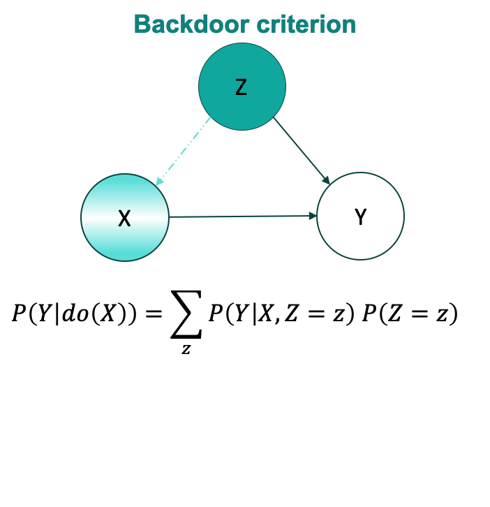
This diagram illustrates the classic confounding structure. The variable Z opens a "backdoor path" from X to Y (X ← Z → Y) that does not represent a causal effect of X on Y. To find the causal effect, we must "close" this backdoor by adjusting for Z. The formula shows how this adjustment is performed.

When a set of variables $Z$ satisfies the backdoor criterion, the causal effect of $X$ on $Y$ is given by the backdoor adjustment formula:

P (Y = y ∣ d o (X = x)) = z \sum P (Y = y ∣ X = x, Z = z) P (Z = z)

Let's break this down:

$P (Y = y ∣ X = x, Z = z)$ is the probability of a specific outcome within a single stratum. You've already worked with this: it's the satisfaction rate for a given studio among clients who chose a specific package type.
$P (Z = z)$ is the marginal probability of that stratum in the overall population. It acts as a weight.
The formula computes a weighted average. It takes the outcome rate from each subgroup ( $z$ ) and weights it by that subgroup's prevalence in the total population. This process creates a synthetic distribution where the treatment $X$ is no longer correlated with the confounder $Z$ , allowing the true causal effect to emerge.

Deriving the Formula

For an investigator with your statistical background, it's not enough to just have the formula; you should understand where it comes from. It isn't arbitrary—it is derived directly from the fundamental rules of do-calculus. The following article provides a superb, step-by-step derivation.

Do-calculus adventures! Exploring the three rules of ... - Andrew Heiss

This article demystifies do-calculus and shows how the backdoor formula is logically derived from its three core rules. This will give you a foundational understanding of why the adjustment works.

Please read the section titled Deriving the backdoor adjustment formula. The author starts with the target causal quantity, P(y | do(x)), and masterfully applies marginalization followed by Rule 2 and Rule 3 of do-calculus. Observe how these rules systematically eliminate the do() operators, transforming an interventional query into a statistical expression you can calculate entirely from your case files (observational data).

Case Solved: The True Effect of Studio Choice

Let's put this formula into action with the data from our studio case. Suppose your investigation yielded the following numbers for 1000 clients:

Package (Z)	Studio (X)	Satisfied (Y=1)	Not Satisfied (Y=0)	Total	Satisfaction Rate
Basic	V&V	81	9	90	90%
	S&S	272	108	380	71.6%
Premium	V&V	192	48	240	80%
	S&S	224	66	290	77.2%

The confounded, overall satisfaction rate for Velvet & Vellum is $(81 + 192) / (90 + 240) = 273/330 \approx 82.7%$ , while for Satin & Steel it's $(272 + 224) / (380 + 290) = 496/670 \approx 74%$ . This suggests V&V is better, but this is still just an association. Let's find the true causal effect.

1. Calculate $P (Z = z)$ :

Total clients with Basic package: $90 + 380 = 470$ . So, $P (Z = Basic) = 470/1000 = 0.47$ .
Total clients with Premium package: $240 + 290 = 530$ . So, $P (Z = Premium) = 530/1000 = 0.53$ .

2. Find $P (Y = 1∣ X = x, Z = z)$ :
These are the stratum-specific rates from the table:

$P(Y=1 | X=\text{V&V}, Z=\text{Basic}) = 0.90$
$P(Y=1 | X=\text{V&V}, Z=\text{Premium}) = 0.80$
$P(Y=1 | X=\text{S&S}, Z=\text{Basic}) = 0.716$
$P(Y=1 | X=\text{S&S}, Z=\text{Premium}) = 0.772$

3. Apply the Backdoor Adjustment Formula:

For Velvet & Vellum (V&V):

\begin{align*} P(Y=1 | do(X=\text{V&V})) &= \sum_{z} P(Y=1 | X=\text{V&V}, Z=z) P(Z=z) \\ &= P(Y=1|X=\text{V&V}, Z=\text{Basic})P(Z=\text{Basic}) + P(Y=1|X=\text{V&V}, Z=\text{Premium})P(Z=\text{Premium}) \\ &= (0.90 \times 0.47) + (0.80 \times 0.53) \\ &= 0.423 + 0.424 = 0.847 \end{align*}

The true causal effect of choosing Velvet & Vellum is an 84.7% satisfaction rate.

For Satin & Steel (S&S):

\begin{align*} P(Y=1 | do(X=\text{S&S})) &= (0.716 \times 0.47) + (0.772 \times 0.53) \\ &= 0.3365 + 0.4092 = 0.7457 \end{align*}

The true causal effect of choosing Satin & Steel is a 74.6% satisfaction rate.

The calculation confirms our earlier intuition from stratification: Velvet & Vellum is indeed the superior studio. The causal difference in satisfaction is approximately 10.1 percentage points.

From Theory to Practice: Adjustment Methods

Calculating by hand is feasible for a simple case, but for complex investigations with many confounders (some continuous), we use statistical methods that operationalize the backdoor adjustment.

The following video provides an excellent intuitive overview of identifying and closing backdoor paths.

Causality: Closing Back Doors

This video from "Econometrics, Causality, and Coding with Dr. HK" offers a clear, conceptual framework for thinking about backdoor paths and why closing them is the central task of causal identification from observational data.

First, watch the explanation of front and back doors to solidify the concept of different paths on a causal diagram. Then, observe how this logic is applied in the more complex example of wine and lifespan, where the narrator identifies multiple paths and discusses which variables to adjust for to close the backdoors.

The most common practical methods are regression adjustment and propensity score methods like Inverse Probability Weighting (IPW). The article below demonstrates these techniques with code, showing how the abstract formula translates into powerful data analysis tools.

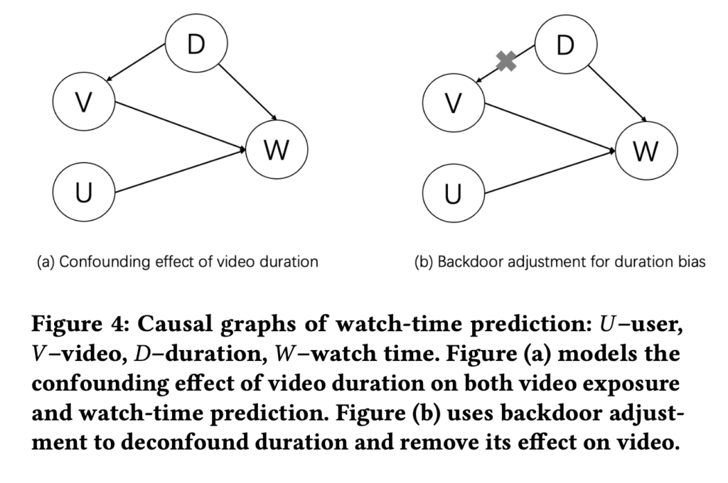
This pair of causal graphs from a real-world study on video recommendations illustrates our goal perfectly. In (a), Duration (D) is a confounder, creating a backdoor path D → V → W. In (b), backdoor adjustment is used to block the path from D to V, isolating the true causal effect of video attributes on watch time.

Ways to close backdoors in DAGs

Now that you have the theory, this article demonstrates two powerful practical methods for performing backdoor adjustment in a real data analysis scenario: Inverse Probability Weighting (IPW) and Matching.

Focus on two main sections. First, read about Adjustment using IPW. Note the two-step process: modeling the probability of treatment (propensity scores), then using these scores to weight the data. Next, review the section on Adjustment using matching, which presents an alternative way to create a comparable pseudo-population. These are the tools you would use in a more complex investigation.

Conclusion

You have now added a powerful and precise instrument to your detective toolkit. By moving from identifying problems to formally correcting for them, you can now answer not just what happened, but why, and quantify the causal impact of any single factor.

Key Takeaways:

The do-operator, $P (Y ∣ d o (X))$ , represents the causal effect of an intervention, which is distinct from the observational association $P (Y ∣ X)$ .
The backdoor adjustment formula is our primary tool for calculating $P (Y ∣ d o (X))$ from observational data, provided we can measure and adjust for a set of variables $Z$ that block all confounding paths.
The formula works by creating a weighted average of stratum-specific outcomes, re-weighting them by their prevalence in the overall population.
In practice, this adjustment is performed using methods like multiple regression, matching, or inverse probability weighting.

Preview of the Next Investigation: The Hidden Pathway

You've learned to handle confounding by adjusting for the confounder, Z. But what if Z is hidden? What if the "Package Type" data was lost or never recorded? Are we powerless? Not at all. In our next case, you will learn about the front-door adjustment, a clever and non-obvious technique for estimating a causal effect even when the main confounder is unobserved, provided we can measure a mediating variable that lies on the causal path between the treatment and the outcome. The investigation continues.

Recommended resources