Welcome to the next lesson in our journey through Operating Systems. In our previous session, we conceptually compared three fundamental CPU scheduling algorithms: First-Come, First-Served (FCFS), Shortest Job First (SJF), and Round Robin (RR). We explored their mechanisms and the qualitative trade-offs they make between performance, fairness, and complexity.
Today, we transition from the conceptual to the practical. Our goal is to analyze a given workload to determine which scheduling algorithm minimizes average waiting time. You will act as a system performance analyst, taking a set of processes and crunching the numbers to see how each scheduling choice impacts efficiency. This hands-on, problem-solving approach is central to understanding why schedulers are designed the way they are and will be a great application of the theory we've covered.
We will start by solidifying the key performance metrics, then work step-by-step through a concrete problem, and finally, you'll get a chance to test your skills on a new workload.
The Toolkit for Analysis
To compare algorithms, we need objective criteria. In the context of scheduling, the most common metrics are Turnaround Time and Waiting Time. Let's ensure we have precise definitions for these.
CPU Scheduling in Operating Systems
This article from GeeksforGeeks provides clear, concise definitions of the key terminologies we'll be using for our calculations.
Please read the section Terminologies Used in CPU Scheduling. Focus on the definitions and formulas for Turnaround Time and Waiting Time. Notice the simple relationship between them: Waiting Time = Turnaround Time – Burst Time.
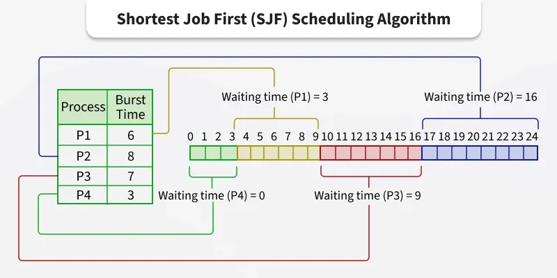
Our primary tool for visualizing the execution of processes will be the Gantt chart. It's a bar chart that illustrates a schedule over time, showing the start and finish times for each process. Seeing the execution flow laid out visually makes calculating the metrics significantly easier.
The Workload: A Practical Challenge
Now, let's introduce the set of processes we will analyze throughout this lesson. Your task, as posed in the problem below, is to calculate the average waiting time for this workload under four different scheduling algorithms:
- First-Come, First-Served (FCFS)
- Shortest Job First (SJF) - Non-Preemptive
- Shortest Remaining Time First (SRTF) - Preemptive SJF
- Round Robin (RR)
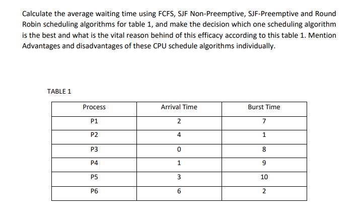
Here is the data in a more accessible format:
| Process | Arrival Time | Burst Time |
|---|---|---|
| P1 | 2 | 7 |
| P2 | 4 | 1 |
| P3 | 0 | 8 |
| P4 | 1 | 9 |
| P5 | 3 | 10 |
| P6 | 6 | 2 |
Guided Calculation Workshop
Solving these problems is a methodical process of building a Gantt chart and then using it to derive the metrics. The following video demonstrates this manual calculation technique for a similar problem. Watching it will give you a strong sense of the workflow we're about to apply.
EASY-HOW-TO CPU Scheduling Algorithm (FCFS, SJF, Non-Preemptive Priority, and RR) Eval (Manual)
This video by Blancaflor Arada provides a clear, step-by-step walkthrough of how to manually evaluate scheduling algorithms.
Watch the initial setup from the beginning. The instructor introduces a problem and calculates the total burst time, which is a useful sanity check to ensure your final Gantt chart's total length is correct. For our problem, the total burst time is 7+1+8+9+10+2 = 37.
Now, let's apply this process to our workload.
1. First-Come, First-Served (FCFS) Analysis
In FCFS, processes are served strictly in the order they arrive. If two processes arrive at the same time, we'll break the tie using the process ID (P1 before P2, etc.), though in this problem, all arrival times are unique.
-
Execution Order: Based on arrival times, the ready queue will process jobs in this order: P3 (arrives at t=0), P4 (t=1), P1 (t=2), P5 (t=3), P2 (t=4), P6 (t=6).
-
Gantt Chart:
- t=0: P3 arrives and starts executing. It runs for its full burst time of 8.
- t=8: P3 completes. P4, P1, P5, P2, and P6 have all arrived by now. The next to run is P4 (arrived at t=1). P4 runs for 9 units.
- t=17: P4 completes. The next to run is P1 (arrived at t=2). P1 runs for 7 units.
- t=24: P1 completes. The next is P5 (arrived at t=3). P5 runs for 10 units.
- t=34: P5 completes. The next is P2 (arrived at t=4). P2 runs for 1 unit.
- t=35: P2 completes. The final process is P6 (arrived at t=6). P6 runs for 2 units.
- t=37: P6 completes.
The Gantt chart looks like this:
-
Calculations:
- Waiting Time = Completion Time - Arrival Time - Burst Time
| Process | Arrival Time | Burst Time | Completion Time | Turnaround Time (CT-AT) | Waiting Time (TT-BT) |
|---|---|---|---|---|---|
| P1 | 2 | 7 | 24 | 22 | 15 |
| P2 | 4 | 1 | 35 | 31 | 30 |
| P3 | 0 | 8 | 8 | 8 | 0 |
| P4 | 1 | 9 | 17 | 16 | 7 |
| P5 | 3 | 10 | 34 | 31 | 21 |
| P6 | 6 | 2 | 37 | 31 | 29 |
| Total | 102 |
- Average Waiting Time (FCFS):
2. Shortest Job First (SJF) - Non-Preemptive Analysis
In non-preemptive SJF, once a process starts, it runs to completion. When the CPU becomes free, the scheduler chooses the process from the ready queue that has the smallest burst time.
-
Gantt Chart:
- t=0: Only P3 (BT=8) is in the ready queue. It starts running.
- t=8: P3 completes. By now, P1 (BT=7), P2 (BT=1), P4 (BT=9), P5 (BT=10), and P6 (BT=2) have all arrived. The scheduler inspects the ready queue and finds the shortest job: P2 (BT=1). P2 starts running.
- t=9: P2 completes. The shortest job in the ready queue is now P6 (BT=2). P6 starts running.
- t=11: P6 completes. The shortest remaining is P1 (BT=7). P1 starts.
- t=18: P1 completes. The shortest remaining is P4 (BT=9). P4 starts.
- t=27: P4 completes. The only one left is P5 (BT=10). P5 starts.
- t=37: P5 completes.
The Gantt chart looks like this:
-
Calculations:
| Process | Arrival Time | Burst Time | Completion Time | Turnaround Time (CT-AT) | Waiting Time (TT-BT) |
|---|---|---|---|---|---|
| P1 | 2 | 7 | 18 | 16 | 9 |
| P2 | 4 | 1 | 9 | 5 | 4 |
| P3 | 0 | 8 | 8 | 8 | 0 |
| P4 | 1 | 9 | 27 | 26 | 17 |
| P5 | 3 | 10 | 37 | 34 | 24 |
| P6 | 6 | 2 | 11 | 5 | 3 |
| Total | 57 |
- Average Waiting Time (SJF):
3. Shortest Remaining Time First (SRTF) - Preemptive SJF Analysis
This is the preemptive version. The scheduler can interrupt a running process if a new process arrives with a burst time shorter than the remaining time of the current process.
-
Gantt Chart: This requires careful, step-by-step tracking.
- t=0: P3 (BT=8) arrives and starts.
- t=1: P4 (BT=9) arrives. P3 has remaining time 7. Since 7 < 9, P3 continues.
- t=2: P1 (BT=7) arrives. P3 has remaining time 6. Since 6 < 7, P3 continues.
- t=3: P5 (BT=10) arrives. P3 has remaining time 5. Since 5 < 10, P3 continues.
- t=4: P2 (BT=1) arrives. P3 has remaining time 4. Since 1 < 4, P3 is preempted! P2 starts running.
- t=5: P2 completes. The scheduler checks the ready queue: P3 (remaining BT=4), P4 (BT=9), P1 (BT=7), P5 (BT=10). The shortest is P3. P3 resumes.
- t=6: P6 (BT=2) arrives. P3 has remaining time 3. Since 2 < 3, P3 is preempted again! P6 starts running.
- t=8: P6 completes. Scheduler checks ready queue: P3 (rem BT=3), P4 (BT=9), P1 (BT=7), P5 (BT=10). Shortest is P3. P3 resumes.
- t=11: P3 completes. Scheduler checks ready queue: P1 (BT=7), P4 (BT=9), P5 (BT=10). Shortest is P1. P1 starts.
- t=18: P1 completes. Shortest is P4 (BT=9). P4 starts.
- t=27: P4 completes. Only P5 (BT=10) is left. P5 starts.
- t=37: P5 completes.
The Gantt chart looks like this:
-
Calculations:
| Process | Arrival Time | Burst Time | Completion Time | Turnaround Time (CT-AT) | Waiting Time (TT-BT) |
|---|---|---|---|---|---|
| P1 | 2 | 7 | 18 | 16 | 9 |
| P2 | 4 | 1 | 5 | 1 | 0 |
| P3 | 0 | 8 | 11 | 11 | 3 |
| P4 | 1 | 9 | 27 | 26 | 17 |
| P5 | 3 | 10 | 37 | 34 | 24 |
| P6 | 6 | 2 | 8 | 2 | 0 |
| Total | 53 |
- Average Waiting Time (SRTF):
4. Round Robin (RR) Analysis
For Round Robin, we need a time quantum. Let's use a time quantum (q) = 3. A process runs for up to 3 time units before being preempted and moved to the back of the ready queue.
-
Gantt Chart:
- t=0: P3 (BT=8) arrives and starts.
- t=3: P3's quantum expires. It is preempted (remaining BT=5) and moved to the back of the queue. At t=3, the ready queue is [P4, P1, P5, P3]. P4 starts.
- t=6: P4's quantum expires. It is preempted (remaining BT=6). At t=6, P2 and P6 have arrived. The ready queue is now [P1, P5, P2, P6, P4]. P1 starts.
- t=9: P1's quantum expires (remaining BT=4). Queue: [P5, P2, P6, P4, P1]. P5 starts.
- t=12: P5's quantum expires (remaining BT=7). Queue: [P2, P6, P4, P1, P5]. P2 starts. It only needs 1 unit.
- t=13: P2 completes. Queue: [P6, P4, P1, P5]. P6 starts. It only needs 2 units.
- t=15: P6 completes. Queue: [P4, P1, P5]. P4 resumes.
- t=18: P4's quantum expires (remaining BT=3). Queue: [P1, P5, P4]. P1 resumes.
- t=21: P1's quantum expires (remaining BT=1). Queue: [P5, P4, P1]. P5 resumes.
- t=24: P5's quantum expires (remaining BT=4). Queue: [P4, P1, P5]. P4 resumes.
- t=27: P4 completes (used its final 3 units). Queue: [P1, P5]. P1 resumes. It only needs 1 unit.
- t=28: P1 completes. Queue: [P5]. P5 resumes.
- t=32: P5's quantum expires (remaining BT=1). Queue: [P5]. P5 resumes.
- t=33: P5 completes. Wait, my math is off. Let's re-calculate the last part.
- t=28: P1 completes. P5 is the only one left. It has 4 units remaining. It runs to completion.
- t=28 -> t=32. P5 completes. Total time is 32. This doesn't match the total burst time of 37. Let's retrace RR carefully.
Let's try again:
- t=0: P3 starts (BT=8). Ready Queue: [].
- t=1: P4 arrives. Q: [P4].
- t=2: P1 arrives. Q: [P4, P1].
- t=3: P3 preempted (rem BT=5). P5 arrives. Q: [P4, P1, P5, P3]. P4 starts (BT=9).
- t=4: P2 arrives. Q: [P4, P1, P5, P3, P2].
- t=6: P4 preempted (rem BT=6). P6 arrives. Q: [P1, P5, P3, P2, P6, P4]. P1 starts (BT=7).
- t=9: P1 preempted (rem BT=4). Q: [P5, P3, P2, P6, P4, P1]. P5 starts (BT=10).
- t=12: P5 preempted (rem BT=7). Q: [P3, P2, P6, P4, P1, P5]. P3 resumes (rem BT=5).
- t=15: P3 preempted (rem BT=2). Q: [P2, P6, P4, P1, P5, P3]. P2 starts (BT=1).
- t=16: P2 completes. Q: [P6, P4, P1, P5, P3]. P6 starts (BT=2).
- t=18: P6 completes. Q: [P4, P1, P5, P3]. P4 resumes (rem BT=6).
- t=21: P4 preempted (rem BT=3). Q: [P1, P5, P3, P4]. P1 resumes (rem BT=4).
- t=24: P1 preempted (rem BT=1). Q: [P5, P3, P4, P1]. P5 resumes (rem BT=7).
- t=27: P5 preempted (rem BT=4). Q: [P3, P4, P1, P5]. P3 resumes (rem BT=2).
- t=29: P3 completes. Q: [P4, P1, P5]. P4 resumes (rem BT=3).
- t=32: P4 completes. Q: [P1, P5]. P1 resumes (rem BT=1).
- t=33: P1 completes. Q: [P5]. P5 resumes (rem BT=4) and runs to completion.
- t=37: P5 completes. This works. The total time is 37.
The Gantt chart looks like this:
-
Calculations:
| Process | Arrival Time | Burst Time | Completion Time | Turnaround Time (CT-AT) | Waiting Time (TT-BT) |
|---|---|---|---|---|---|
| P1 | 2 | 7 | 33 | 31 | 24 |
| P2 | 4 | 1 | 16 | 12 | 11 |
| P3 | 0 | 8 | 29 | 29 | 21 |
| P4 | 1 | 9 | 32 | 31 | 22 |
| P5 | 3 | 10 | 37 | 34 | 24 |
| P6 | 6 | 2 | 18 | 12 | 10 |
| Total | 112 |
- Average Waiting Time (RR):
The Verdict
Let's compile our results into a final comparison table.
| Scheduling Algorithm | Average Waiting Time |
|---|---|
| First-Come, First-Served | 17.0 |
| Shortest Job First (Non-Pre.) | 9.5 |
| Shortest Rem. Time (Pre.) | 8.83 |
| Round Robin (q=3) | 18.67 |
For this specific workload, SRTF (Preemptive SJF) provides the lowest average waiting time. This result is consistent with the theory we discussed in the previous lesson: SJF is provably optimal for minimizing average waiting time. The preemptive version (SRTF) performs even better because it can capitalize on newly arrived short jobs to prevent them from waiting behind a longer, currently running job.
FCFS and Round Robin performed the worst on this metric. This highlights the convoy effect in FCFS and the overhead/fairness trade-off in RR. While RR ensures no process waits too long for its first response (good for interactivity), it doesn't optimize for total time spent waiting in the queue.
Put Your Knowledge to the Test
Now it's your turn. Below is a new workload. Your task is to calculate the average waiting time (or average response time, which is equivalent to turnaround time here) for FCFS, Round Robin (with a time slice of 10), and SRTF.
| Job | Length (Burst Time) | Arrival Time |
|---|---|---|
| 0 | 85 | 0 |
| 1 | 30 | 10 |
| 2 | 35 | 10 |
| 3 | 20 | 80 |
| 4 | 50 | 85 |
Take some time to draw the Gantt charts and compute the metrics for each algorithm. This is an excellent exercise to solidify your understanding. Once you have your answers, you can check your work against the provided solution.
CS372: Solutions for Homework 9
This document contains the solution to the problem above. Use it to verify your calculations.
Review the solution for Problem 4. The table summarizes the completion and response times for each job under FIFO (FCFS), RR, and SRTF. Note that "Response Time" in this document is calculated as Completion Time - Arrival Time, which is how we defined Turnaround Time. You can find the average waiting time by subtracting the burst time from the turnaround time for each process and then averaging. The conclusion remains the same: SRTF provides the best performance on this metric.
Conclusion
In this lesson, you've put theory into practice by quantitatively analyzing the performance of CPU scheduling algorithms. You have seen firsthand how different scheduling policies lead to vastly different outcomes for the same set of processes.
The key takeaways are:
- Gantt charts are an indispensable tool for visualizing process execution and calculating performance metrics.
- Average Waiting Time is a critical metric for evaluating scheduler efficiency, especially in batch systems.
- Shortest Job First (SJF), and particularly its preemptive version SRTF, is optimal for minimizing average waiting time by prioritizing short jobs.
- The choice of algorithm always involves trade-offs. While SRTF won on this metric, an algorithm like Round Robin might be preferred in an interactive system where fairness and response time are more important than minimizing total wait.
We have now explored how the OS manages multiple processes and decides which one gets the CPU. But how do these independent processes coordinate and communicate with each other? In our next lesson, we will dive into the world of Inter-Process Communication (IPC), exploring mechanisms like pipes, shared memory, and message passing that allow processes to work together.