In our last lesson, we saw how the fork(), exec(), and wait() system calls work in concert to create and manage processes. This raised a crucial question: in a multitasking system with many processes ready to run, how does the operating system decide which one gets the CPU? This lesson delves into the answer by exploring the world of CPU scheduling.
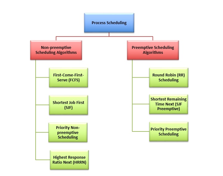
Our goal is to compare the fundamental CPU scheduling algorithms that form the basis of modern operating systems. We'll start by establishing the primary distinction between preemptive and non-preemptive scheduling. Then, we will examine three classic algorithms:
- First-Come, First-Served (FCFS)
- Shortest Job First (SJF)
- Round Robin (RR)
By the end of this lesson, you will understand how each algorithm works, its defining characteristics, and the critical trade-offs it makes in terms of performance, fairness, and complexity.
Preemptive vs. Non-Preemptive Scheduling
At its core, every scheduling algorithm must adhere to one of two philosophies: non-preemptive or preemptive.
- Non-preemptive scheduling is cooperative. Once a process is given the CPU, it keeps it until it voluntarily releases it—either by finishing its task or by performing an I/O operation.
- Preemptive scheduling is forceful. The operating system can interrupt a running process, take the CPU away, and give it to another process. This is typically done using a hardware timer.
This single difference has profound implications for system responsiveness, fairness, and protection against misbehaving programs.
The video below offers a clear and concise explanation of this core distinction and introduces the concept of a "quantum," which is fundamental to preemptive scheduling.
This segment from a video by Jacob Sorber clearly defines and contrasts cooperative (non-preemptive) and preemptive scheduling.
Please watch the section from the beginning that explains the two main varieties of schedulers and why modern systems favor the preemptive approach.
The table in the following document also provides a useful side-by-side comparison of their characteristics.
Unit IV – CPU Scheduling and Algorithm
This document provides a concise table comparing the two scheduling types.
Find the table titled Basis for Comparison and review the key differences regarding interrupts, starvation, and overhead.
In essence, non-preemptive schedulers are simpler but risk having the entire system performance dictated by a single long-running or uncooperative process. Preemptive schedulers are more complex but provide the fairness and responsiveness expected of modern interactive operating systems.

First-Come, First-Served (FCFS): The Simple but Flawed Approach
First-Come, First-Served (FCFS) is the most straightforward scheduling algorithm. It operates exactly as its name implies: processes are served in the order they arrive in the ready queue. It is a non-preemptive algorithm.
- Mechanism: Implemented with a simple First-In, First-Out (FIFO) queue. When the current process releases the CPU, the process at the head of the queue gets it next.
- Advantage: Very simple to understand and implement.
- Disadvantage: FCFS can lead to poor performance due to the convoy effect. If a long, CPU-bound process arrives just before several short, I/O-bound processes, the short processes are forced to wait, leaving I/O devices idle. This results in poor utilization of system resources and high average waiting times.
The following video provides an excellent intuitive explanation of FCFS and visualizes the convoy effect.
The Fancy Algorithms That Make Your Computer Feel Smoother
This video from Core Dumped explains the FCFS algorithm and its primary weakness.
Watch from the introduction to understand the basic mechanism. Then, jump to the segment on the convoy effect to see why this simple algorithm is often inefficient.
To see this in practice, let's look at a concrete example.
Unit IV – CPU Scheduling and Algorithm
This document contains worked examples of scheduling algorithms. The FCFS examples demonstrate the calculation of waiting and turnaround times.
Please read the section on First Come First Serve (FCFS). Pay close attention to Example 2. Notice how the long burst time of process P1 (24ms) forces P2 and P3 to wait, leading to a high average waiting time of 17ms, even though P2 and P3 are very short. This is a classic demonstration of the convoy effect.
Shortest Job First (SJF): An Optimal but Impractical Solution
To address the convoy effect, we can use the Shortest Job First (SJF) algorithm. The core idea is to prioritize processes with the shortest upcoming CPU burst.
SJF can be either non-preemptive or preemptive:
- Non-preemptive SJF: When the CPU becomes free, the scheduler selects the process with the shortest next CPU burst from the entire ready queue.
- Preemptive SJF (Shortest Remaining Time First - SRTF): This is a more aggressive version. If a new process arrives in the ready queue with a CPU burst shorter than the remaining time of the currently executing process, the scheduler preempts the current process and runs the new, shorter one.
Advantages & Disadvantages:
- Advantage: SJF (specifically, the preemptive SRTF variant) is provably optimal in minimizing the average waiting time for a given set of processes.
- Disadvantage 1 (Impracticality): Its greatest weakness is that it's impossible to implement perfectly. There is no way to know the exact length of a process's next CPU burst in advance. Schedulers must rely on predicting future behavior based on past performance, typically using an exponential average of previous burst lengths.
- Disadvantage 2 (Starvation): SJF can lead to starvation. A process with a long CPU burst might never get to run if there is a continuous stream of shorter jobs arriving.
This video provides an excellent overview of SJF, including the formula used for prediction.
The Fancy Algorithms That Make Your Computer Feel Smoother
This video explains the logic behind SJF, its optimality, the prediction problem, and the risk of starvation.
Watch from the introduction to SJF to understand how it works and how future CPU bursts are estimated. Then, continue watching the segment from on starvation to see the major drawback of this approach.
The exponential average formula for predicting the next burst length, , is:
Where:
- is the duration of the actual -th CPU burst.
- was the predicted duration for that -th burst.
- is a weighting factor between 0 and 1.
Now, let's compare the non-preemptive and preemptive versions with a worked example.
Unit IV – CPU Scheduling and Algorithm
This section provides a direct comparison between non-preemptive SJF and preemptive SRTF using the same set of processes.
Read the section on Shortest Job First (SJF). Work through Example-01 (non-preemptive) and then Example-02 (preemptive). Notice how both the average waiting time and turnaround time are lower in the preemptive (SRTF) case because the scheduler can interrupt a running process to service a newly arrived, shorter job.
Round Robin (RR): Preemption for Fairness
While SJF optimizes for average waiting time, it can be unfair to long processes. For interactive systems where responsiveness is key, a different approach is needed. Round Robin (RR) is a preemptive algorithm designed specifically for time-sharing environments.
- Mechanism: RR is essentially FCFS with preemption. Each process is allowed to run for a small, fixed time interval called a time quantum (or time slice), typically 10-100 milliseconds.
- Execution Flow:
- The scheduler picks the first process from the ready queue and lets it run.
- If the process finishes its CPU burst before the time quantum expires, it releases the CPU voluntarily.
- If the process is still running when the quantum expires, a hardware timer triggers an interrupt, and the OS preempts the process, placing it at the tail of the ready queue.
- The scheduler then proceeds to the next process at the head of the queue.
The performance of RR is highly dependent on the size of the time quantum:
- Too large: RR degenerates into FCFS, and responsiveness suffers.
- Too small: The overhead from frequent context switching becomes significant, reducing overall throughput.
The Fancy Algorithms That Make Your Computer Feel Smoother
This section of the video uses a clear animation to demonstrate the Round Robin algorithm and discusses the critical trade-off involved in choosing a time quantum.
Watch from the explanation of Round Robin. Pay attention to the animated queue and the discussion on how turnaround time is affected by the quantum size.
Let's see the calculations for RR in action.
Unit IV – CPU Scheduling and Algorithm
This part of the document provides a step-by-step example of the Round Robin algorithm.
Read the section on Round Robin Scheduling. Follow the Gantt chart and calculations in Example-01. Tracing how each process runs for the time quantum (2 units) and is then moved to the back of the ready queue is key to understanding its behavior.
Conclusion
In this lesson, we have dissected three foundational CPU scheduling algorithms, each embodying a different set of trade-offs. There is no single "best" algorithm; the choice depends entirely on the system's goals, whether that's maximizing throughput, minimizing response time, or ensuring fairness.
Here is a summary of our comparison:
| Algorithm | Type | Key Idea | Advantages | Disadvantages |
|---|---|---|---|---|
| First-Come, First-Served (FCFS) | Non-Preemptive | Process jobs in the order they arrive. | Simple to implement. | Suffers from the convoy effect; high average waiting time. |
| Shortest Job First (SJF) | Preemptive or Non-Preemptive | Execute the job with the shortest next CPU burst. | Provably optimal for average waiting time. | Impossible to predict burst length; can lead to starvation of long jobs. |
| Round Robin (RR) | Preemptive | Give each job a small time slice (quantum). | Fair and responsive; good for time-sharing. | Performance is sensitive to quantum size; context switch overhead. |
You've now grasped the fundamental principles that govern how an OS allocates its most critical resource: the CPU.
In our next lesson, we will apply this knowledge in a more practical context. We will move from simply comparing algorithms to analyzing a given workload to determine which scheduling algorithm minimizes average waiting time, a common exercise in system performance tuning.