Recommended resources
The freely available resources this lesson will direct you to.
Introduction
In our last lesson, we confronted the degradation problem: the paradoxical phenomenon where adding more layers to a "plain" network leads to higher training error. We established this is an optimization failure, not a lack of representational power. We even proved, by construction, that a deeper network should perform at least as well as a shallower one by having the extra layers learn identity mappings. The fact that optimizers fail to find this solution, coupled with the chaotic loss landscapes of very deep plain networks, sets the stage for a powerful architectural solution.
This lesson dissects that very solution: the residual connection. We will explore how this simple yet profound idea, introduced in the "Deep Residual Learning for Image Recognition" paper, elegantly solves the degradation problem. We will see how reframing the learning objective within a layer—from learning a new function to learning a small change—makes optimization tractable and unlocks the ability to train truly deep networks.
Part 1: Reframing the Problem - Learning the Residual
The core insight behind Residual Networks (ResNets) is to change what the building blocks of the network are asked to learn. Instead of asking a set of layers to approximate a desired underlying mapping, , we instead ask them to learn a residual mapping, .
The desired mapping is then recast as the sum of the input and this new residual function:
The block of layers now only needs to learn the difference, . This change is motivated by the degradation problem itself.
To build intuition, consider a task from computer graphics: image super-resolution. The goal is to take a low-resolution image, , and produce a high-resolution version, . In many cases, the high-res output is very similar to an upsampled version of the low-res input. Most of the information is already present. A standard network would try to generate the entire high-res image from scratch. A residual network, however, would learn the "residual"—the fine details and high-frequency information that need to be added to the upsampled input to produce the final image. This is often a much easier task.
Professor Steve Brunton provides an excellent visual explanation of this idea.
Residual Networks (ResNet) [Physics Informed Machine Learning]
This video from the "Physics Informed Machine Learning" series provides a great intuitive motivation for residual networks.
Watch the first segment from the introduction. Pay close attention to the super-resolution example and the idea of modeling the difference or the delta changes from input to output.
This reframing directly addresses the optimization paradox we discussed. Let's formalize this with a Socratic question.
Socratic Question: In the previous lesson, we established that a key challenge for very deep plain networks is learning an identity mapping () for the additional layers. Using the residual formulation, , what must the network learn for to make the overall block an identity mapping? Why is learning this easier for a typical stack of layers initialized with small random weights?
Answer
To make $H(\mathbf{x}) = \mathbf{x}$, the residual function must become the zero function, $F(\mathbf{x}) = \mathbf{0}$.This is significantly easier for a network to learn. As we've discussed, standard weight initialization schemes (e.g., from a zero-mean Gaussian) and regularization techniques like L2 weight decay inherently bias the network's layers toward learning functions with small outputs. Driving the output of a block to zero is a natural tendency for the optimizer. In contrast, learning the identity function requires the weights to learn a very specific, non-zero structure, which is a much harder optimization target.
The original ResNet paper formalizes this exact hypothesis.
Deep Residual Learning for Image Recognition
Let's dive into the original paper by Kaiming He et al. to see how they presented this core concept.
First, read the two paragraphs that introduce the concept, starting from "In this paper, we address the degradation problem...". This section formally defines the residual mapping F(\mathbf{x}) := H(\mathbf{x}) - \mathbf{x} and the hypothesis that it's easier to optimize. Next, read the section "3.1. Residual Learning". Focus on the paragraph "The degradation problem suggests...". This directly states the argument from our Socratic question: if identity mappings are optimal, the solver can simply drive the weights toward zero.
Part 2: The Architectural Innovation - The Skip Connection
This reformulation from to is realized through a simple and elegant architectural element: the shortcut connection, often called a skip connection.
This is a direct connection that bypasses one or more layers, carrying the input forward and adding it to the output of the layers it skips.
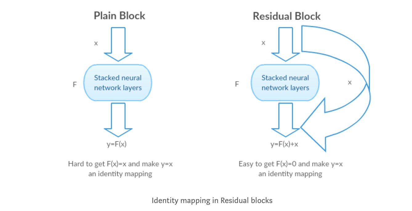
The stacked layers (e.g., two CONV -> BN -> ReLU layers) are responsible for learning the residual function . The skip connection simply performs an identity mapping, and its output is added element-wise to the output of the stacked layers. The final output of the block is then:
From a systems engineering perspective, this is a brilliant design. The element-wise addition is computationally negligible, adding virtually no parameters or FLOPs to the network. Yet, its impact on trainability is enormous.
The textbook "Dive into Deep Learning" provides a great discussion on how this structure creates nested function classes. By adding layers that can default to being identity mappings, we ensure that a deeper network's set of possible functions strictly contains that of a shallower one (). This guarantees that adding depth can only improve the model's potential.
8.6. Residual Networks (ResNet) and ResNeXt
This chapter from "Dive into Deep Learning" provides a very clear explanation of the residual block's mechanics and the theory behind it.
First, read the section on Function Classes. This provides the theoretical justification for why we want architectures where deeper models are guaranteed to be at least as expressive as shallower ones. Next, read the section on Residual Blocks. It clearly illustrates how the shortcut connection implements the residual learning idea. Notice the diagram which is similar to the one above. The provided code snippets show how simple the implementation is in a modern framework.
Part 3: The Empirical Solution and Deeper Intuition
The theory is elegant, but the definitive proof is in the results. By introducing residual connections, the authors of the ResNet paper were able to completely reverse the degradation trend.
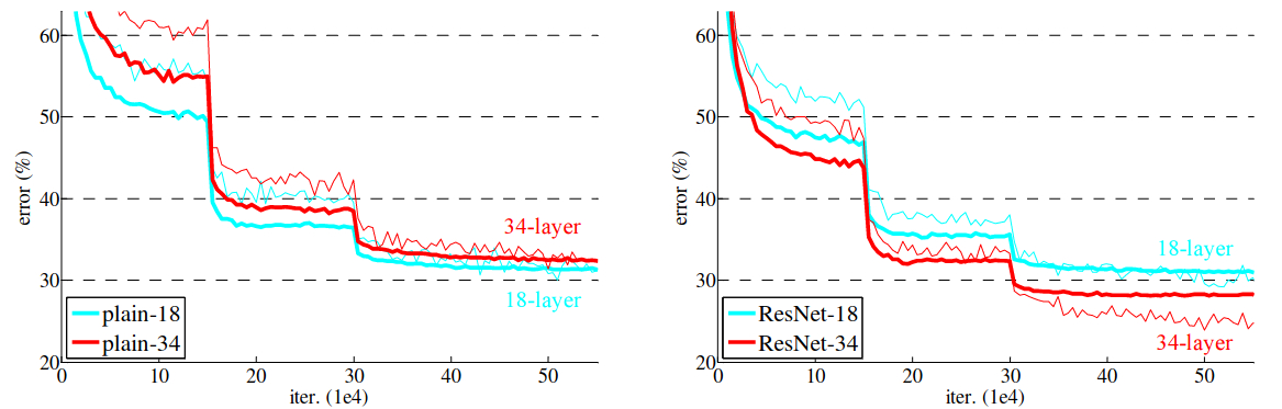
The image above is one of the most famous figures in deep learning. The left plot shows the degradation problem we studied last lesson: the deeper plain-34 network has higher error than the plain-18 network. The right plot shows the effect of adding residual connections. The situation is completely reversed: the ResNet-34 is now clearly superior to the ResNet-18, achieving much lower error. This demonstrates that the optimization problem has been solved and the network is now gaining accuracy from increased depth.
Let's hear this explained and then read the paper's own analysis.
[Classic] Deep Residual Learning for Image Recognition (Paper Explained)
We return to Yannic Kilcher's explanation of the paper.
Watch the segment explaining the core idea of the residual connection and how it biases the network towards the identity function. Then, watch the walkthrough of the experimental results, where he discusses the exact plot shown above. Finally, briefly watch from this comparison showing that as you go even deeper (50, 110 layers), ResNets continue to improve while plain networks get worse.
Deep Residual Learning for Image Recognition
Now, let's read the paper's own description of their groundbreaking results.
Read the section titled "Residual Networks" in Section 4.1. The authors present three major observations from their results, confirming that residual learning solves the degradation problem and allows for accuracy gains from increased depth.
A Connection to Numerical Methods
Your engineering background might appreciate another powerful intuition for ResNets. Consider the Euler method for numerical integration of an ordinary differential equation (ODE), where you want to find the state of a system over time. The state at the next time step is the current state plus a small change:
Here, represents the "change" or the derivative. This looks remarkably similar to a residual block, where each block computes a small update to the representation as it passes through the network. This perspective views a deep ResNet as a discretized solver for an underlying continuous transformation.
Professor Brunton explains this connection beautifully.
Residual Networks (ResNet) [Physics Informed Machine Learning]
Let's return to Steve Brunton's video for this final piece of intuition.
Watch the segment from "one of the ways I think about res Nets". He explicitly draws the parallel between the residual update rule and numerical integrators like Euler integration.
This perspective also helps explain why skip connections are so critical for backpropagation. They create a direct, linear "superhighway" for the gradient to flow backwards through the layers, mitigating the vanishing gradient problem that plagues very deep sequential models. The gradient doesn't have to navigate a long chain of non-linear transformations and multiplications; it can take the shortcut.
This directly results in the smoother loss landscapes we saw in the previous lesson. The skip connection ensures a linear component in the function computed by each block, which prevents the overall loss surface from becoming as chaotic and non-convex as it does in plain deep networks.
Conclusion
In this lesson, we have seen how a simple and computationally cheap architectural change—the skip connection—solves the profound optimization challenges of training very deep networks. By reframing the learning task from approximating a complete function to approximating a small residual, ResNets make it trivial for layers to learn identity mappings, thereby resolving the degradation paradox.
Key Takeaways:
- Residual Learning: Instead of learning a mapping , residual blocks learn a residual . The output is formed by .
- Skip Connections: This is implemented architecturally with a "skip" or "shortcut" connection that adds the block's input to its output.
- Solving Degradation: This formulation makes learning an identity map trivial (by learning ), which solves the optimization paradox. Empirically, deeper ResNets have lower error than shallower ones.
- Improved Optimization: Skip connections provide a direct path for gradient flow during backpropagation and lead to smoother, more navigable loss landscapes, which is why optimizers can successfully train these networks.
- Numerical Intuition: A ResNet can be viewed as a numerical integrator (like Euler's method), where each block computes a small update to the feature representation.
Preview of the Next Module:
With ResNets, we have reached a pinnacle in the design of deep convolutional networks for vision. We've seen how to effectively extract hierarchical features from images. However, CNNs are inherently local. What if we want to model relationships between pixels that are far apart, or between words in a sentence? This requires a mechanism that can weigh the importance of different parts of the input regardless of their position. In our next module, we will introduce this mechanism: Attention, which forms the heart of the revolutionary Transformer architecture.