Understanding RNN Architecture and the Vanishing/Exploding Gradient Problem

Introduction

In our last lesson, we saw how residual connections conquered the degradation problem in very deep spatial architectures like CNNs. We noted that these skip connections create "highways" for gradients, preventing them from vanishing as they propagate through many layers. This insight is crucial as we now pivot from spatial data to a new domain: sequential data.

Tasks involving language, financial time series, or physics simulations require models that can understand context, remember past events, and handle inputs of variable length. A standard feedforward network, which processes each input independently, is fundamentally unsuited for this. This lesson introduces the Recurrent Neural Network (RNN), an architecture designed from the ground up to model sequences by incorporating a notion of memory. We will dissect its architecture and then uncover its critical flaw: the very mechanism that gives it memory also makes it notoriously difficult to train on long sequences, leading to the infamous vanishing and exploding gradient problems.

Part 1: Modeling Sequences with State

Imagine trying to predict the next word in a sentence. The prediction for "sky" in "The clouds are blue, and so is the ___" depends heavily on the word "blue" that appeared much earlier. A model needs a way to maintain information over time. This is the core idea of recurrence.

Unlike a feedforward network, an RNN processes a sequence one element at a time, and at each step, it combines the current input with information from the previous step. This "information" is stored in a hidden state, a vector that acts as the network's memory.

The key architectural features are:

1. Hidden State ($h_t$): A vector that summarizes the sequence up to timestep $t$. It's computed based on the previous hidden state $h_{t-1}$ and the current input $x_t$.
2. Recurrent Connection: The output of the network at one step (the new hidden state) is fed back into itself as an input for the next step. This is the loop shown on the left of the diagram.
3. Parameter Sharing: The same set of weights ($W_{hh}$, $W_{xh}$, $W_{hy}$) are used at every single timestep. The network doesn't learn a new set of weights for each position in the sequence; it learns a single, general update rule. This makes the model efficient and capable of handling sequences of varying lengths.

Let's watch a brief segment from a Stanford lecture that introduces this concept in the context of language modeling.

Part 2: The Mathematical Formulation of a Simple RNN

Let's formalize the computations shown in the diagram. At each timestep $t$, an RNN performs two main calculations:

1. Hidden State Update: The new hidden state $h_t$ is computed by combining the previous state $h_{t-1}$ and the current input $x_t$. This combination passes through an affine transformation followed by a non-linear activation function, typically the hyperbolic tangent ($\tanh$).

   $$h_t=\tanh (W_{hh}{h}_{t-1}+W_{xh}{x}_t+b_h)$$

   Here:

   • $x_t$ is the input vector at time $t$.
   • $h_{t-1}$ is the hidden state vector from the previous time $t-1$.
   • $W_{xh}$ is the weight matrix for the input-to-hidden connection.
   • $W_{hh}$ is the weight matrix for the hidden-to-hidden (recurrent) connection.
   • $b_h$ is the bias for the hidden layer.

2. Output Calculation: The output for the current timestep, $y_t$, is typically computed from the current hidden state $h_t$.

   $$y_t=W_{hy}{h}_t+b_y$$
   • $W_{hy}$ is the weight matrix for the hidden-to-output connection.
   • $b_y$ is the bias for the output layer. The output $y_t$ might then be passed through a softmax function for classification tasks.

To better understand the flow, let's read a short article that details these operations.

Part 3: The Gradient Problem in Time

Training an RNN involves computing a loss (e.g., at the end of the sequence) and using gradients to update the shared weights $W_{hh}$, $W_{xh}$, and $W_{hy}$. Because the same weights are used at every step, the process of backpropagation must also flow backward through time. This is called Backpropagation Through Time (BPTT).

An update to $W_{hh}$ at time $t=1$ affects $h_1$, which in turn affects $h_2$, which affects $h_3$, and so on, all the way to the final loss calculation. The total gradient for a shared weight is the sum of its gradient contributions from every timestep.

This dependency creates a long chain of computations, which brings us to a familiar challenge.

Socratic Question: To calculate the influence of the hidden state at an early time $t$ on the loss computed at a much later time $T$, we must apply the chain rule. What mathematical form will the expression for $\frac{\partial L_T}{\partial h_t}$ take? Given our experience with very deep feedforward networks, what instability might arise from this structure?

This is precisely the vanishing and exploding gradient problem, but manifested in the temporal dimension.

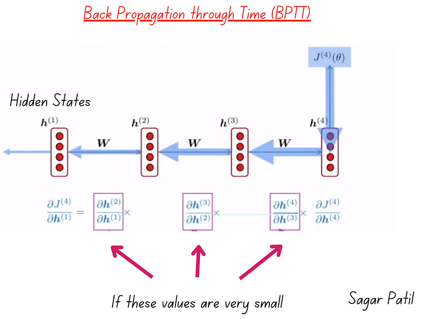
Let's watch a clear, mathematical derivation of this problem.

Part 4: The Mathematical Core of the Instability

As the video explained, the gradient of the loss at time $T$ with respect to a hidden state at an earlier time $t$ is a product of Jacobians:

Let's analyze the Jacobian term $\frac{\partial h_k}{\partial h_{k-1}}$. Starting from our hidden state update equation:

The derivative with respect to $h_{k-1}$ is:

This reveals two key components that are multiplied together at every step back in time:

1. The Activation's Derivative: A diagonal matrix containing the derivatives of the $\tanh$ function. The derivative of $\tanh (z)$ is $1-{\tanh }^2(z)$, which is always between 0 and 1. When the neuron is "saturated" (its input is large and positive or negative), the derivative is close to 0. This term can only shrink the gradient.
2. The Recurrent Weight Matrix $W_{hh}$: This matrix is repeatedly applied. From our study of linear algebra, we know that repeated multiplication of a vector by a matrix $W$ will cause the vector's norm to scale by roughly $({\sigma }_{max}{)}^n$, where ${\sigma }_{max}$ is the largest singular value of $W$ and $n$ is the number of multiplications.

Combining these two factors:

• Vanishing Gradients: If the singular values of $W_{hh}$ are less than 1, or even if they are slightly larger than 1 but the activation derivatives are small, the norm of the overall Jacobian product will be less than 1. When multiplied over many timesteps, the gradient signal shrinks exponentially, effectively "vanishing" to zero. The model becomes unable to learn dependencies between distant timesteps.
• Exploding Gradients: If the singular values of $W_{hh}$ are significantly greater than 1, the gradient norm can grow exponentially, leading to massive, unstable weight updates that derail the training process.

The following article provides a fantastic deep dive into this mathematical reasoning.

While exploding gradients can cause training to fail spectacularly (resulting in NaN loss values), they are the easier problem to solve. We can simply implement gradient clipping: if the norm of the total gradient vector exceeds a certain threshold, we scale it down before the weight update. This is a pragmatic but effective fix.

The vanishing gradient problem is far more insidious. A gradient that has decayed to near-zero contains no useful information. There is no simple trick to "amplify" it back into a meaningful signal. This fundamental limitation is what makes simple RNNs struggle with true long-range dependencies in practice.

Conclusion

In this lesson, we introduced the Recurrent Neural Network as an architecture tailored for sequential data. Its core strength—a recurrent hidden state that acts as memory—is also its greatest weakness during training.

Key Takeaways:

• RNN Architecture: An RNN processes sequences by updating a hidden state $h_t$ based on the previous state $h_{t-1}$ and the current input $x_t$, using the same weights at every timestep.
• Backpropagation Through Time (BPTT): Training involves unrolling the network in time and propagating gradients backward through the entire sequence.
• The Gradient Chain: The recursive nature of the hidden state creates a long product of Jacobian matrices when calculating gradients for distant timesteps.
• Vanishing/Exploding Gradients: This product of matrices causes the gradient signal to either shrink exponentially to zero (vanish) or grow exponentially to infinity (explode).
  • Vanishing occurs when the Jacobians are contractive (e.g., singular values < 1), preventing the model from learning long-term dependencies.
  • Exploding occurs when the Jacobians are expansive (e.g., singular values > 1), causing training instability.
• Asymmetric Problem: Exploding gradients can be managed with gradient clipping, but vanishing gradients represent a fundamental loss of information that cannot be easily recovered.

Preview of the Next Lesson:

The failure of simple RNNs to capture long-range dependencies was a major bottleneck in sequence modeling. This spurred the development of more sophisticated recurrent units designed specifically to combat the vanishing gradient problem. In our next lesson, we will explore Long Short-Term Memory (LSTM) and Gated Recurrent Unit (GRU) networks. We will see how their use of "gates" creates an additive "cell state" pathway, a "gradient highway" that allows information to flow across many timesteps without being degraded by repeated multiplication.