LSTMs and GRUs: Overcoming RNN Limitations

Introduction

In our previous lesson, we unraveled the architecture of a simple Recurrent Neural Network and discovered its critical flaw: the vanishing and exploding gradient problems. We established that the recursive nature of the hidden state, $h_t=f(W_{hh}{h}_{t-1}+...)$, leads to a long product of Jacobian matrices during backpropagation. This multiplicative structure causes the gradient signal to either decay exponentially into oblivion or explode into instability, making it nearly impossible for the network to learn dependencies between distant timesteps.

Today, we will explore the ingenious architectural solutions that broke through this barrier: Long Short-Term Memory (LSTM) and Gated Recurrent Unit (GRU) networks. These models introduce the concept of gates—specialized neural network components that regulate the flow of information. We will dissect how these gates create an alternative, primarily additive pathway for information, allowing gradients to travel across long time horizons without vanishing. This lesson will show you precisely how these mechanisms overcome the limitations of simple RNNs.

Part 1: The Core Idea – A Regulated Information Highway

Before diving into the specific equations, let's build an intuition for the solution. The problem with a simple RNN is that its memory, the hidden state $h_t$, is completely recomputed at every timestep. It's like trying to remember a long story by constantly overwriting your notes with a new summary that includes the latest sentence. Important details from the beginning are likely to get washed out.

LSTMs and GRUs solve this by creating a more persistent "information highway." Imagine a conveyor belt running parallel to the main sequence processing line. This belt can carry information from much earlier timesteps directly to later ones. The innovation lies in creating controllable gates that decide:

1. What old information to remove from the belt.
2. What new information to place on the belt.
3. What information from the belt to use for the current prediction.

To see how this maps to a real-world task, let's start with a brief video that uses a thought experiment to explain this selective memory process.

Part 2: Deconstructing the Long Short-Term Memory (LSTM) Unit

The first and most influential gated architecture is the LSTM, proposed by Hochreiter and Schmidhuber in 1997. An LSTM unit enhances a simple RNN by introducing a cell state ($c_t$) in addition to the hidden state ($h_t$).

• Cell State ($c_t$): This is the information highway or "long-term memory." It's a vector that can carry information across many timesteps with minimal distortion.
• Hidden State ($h_t$): This acts as the "short-term memory" and is the output of the LSTM unit at the current timestep, used for making predictions.

The flow of information into, out of, and within the cell state is controlled by three gates. Each gate is a small neural network (an affine transformation followed by a sigmoid activation function) that outputs a vector of values between 0 and 1. These values act as switches: a value of 0 means "let nothing through," while a value of 1 means "let everything through."

Let's watch a video that introduces the components and then break them down one by one.

As the video explained, the three gates are the Forget Gate, the Input Gate, and the Output Gate.

1. The Forget Gate ($f_t$)

The first step is to decide what information to throw away from the previous cell state, $c_{t-1}$. The forget gate looks at the previous hidden state $h_{t-1}$ and the current input $x_t$ and outputs a number between 0 and 1 for each element in the cell state vector.

A '1' means "completely keep this part of the old memory," while a '0' means "completely forget this part."

2. The Input Gate ($i_t$) and Candidate Memory (${\tilde{c}}_t$)

Next, the LSTM decides what new information to store in the cell state. This has two parts:

• The input gate ($i_t$) decides which values we'll update.
• A $\tanh$ layer creates a vector of new candidate values, ${\tilde{c}}_t$, that could be added to the state.

3. Updating the Cell State ($c_t$)

Now we can update the old cell state $c_{t-1}$ into the new cell state $c_t$. We multiply the old state by the forget gate's output ($f_t$), forgetting the things we decided to forget. Then, we add the new information, scaled by the input gate ($i_t\odot {\tilde{c}}_t$).

This equation is the heart of the LSTM. Notice the additive interaction. We are not nesting functions as in a simple RNN ($h_t=\tanh (W{h}_{t-1}+...)$). Instead, we are adding new information to a modified version of the old state.

4. The Output Gate ($o_t$)

Finally, we need to decide what our output, the hidden state $h_t$, is going to be. The output will be a filtered version of our cell state.

• First, the output gate ($o_t$) decides what parts of the cell state we're going to output.
• Then, we put the cell state through a $\tanh$ function (to squash the values to be between -1 and 1) and multiply it by the output of the output gate.

To see these gates in action with concrete numbers, the StatQuest channel provides an excellent walkthrough.

The article below provides a handy table summarizing all the LSTM equations.

Part 3: How LSTMs Solve the Vanishing Gradient Problem

Now for the crucial question. How does this architecture prevent the gradient from vanishing?

Socratic Question: Consider the cell state update equation: $c_t=f_t\odot c_{t-1}+i_t\odot {\tilde{c}}_t$. If we want to backpropagate the gradient of the loss with respect to the cell state at time $t$, $\frac{\partial L}{\partial c_t}$, back to the cell state at time $t-1$, we need to compute the Jacobian $\frac{\partial c_t}{\partial c_{t-1}}$. What is the simplest, most direct path for this gradient? How does its mathematical form differ from the Jacobian $\frac{\partial h_t}{\partial h_{t-1}}$ in a simple RNN?

The gradient highway is the additive nature of the cell state update. When backpropagating, the gradient can flow from $c_t$ to $c_{t-1}$ directly through the forget gate. The total gradient for a cell state far in the past becomes a product of forget gate activations:

Because the network controls $f_k$, it can learn to set the forget gates to 1 for timesteps where it needs to preserve memory. This creates an uninterrupted channel where the gradient can flow back through time without being repeatedly squashed by a weight matrix and an activation function's derivative. The LSTM architecture doesn't guarantee that gradients won't vanish, but it makes it much easier for the model to learn to preserve long-range dependencies.

The following resource from a Stanford lecture explains this very clearly.

Part 4: Gated Recurrent Unit (GRU) - A Simpler Alternative

The GRU, introduced by Cho et al. in 2014, is a streamlined version of the LSTM that often achieves comparable performance with a simpler structure and fewer parameters. This makes it computationally more efficient, a trait that will likely appeal to your interest in performance systems.

The GRU makes two key changes:

1. Combined State: It merges the cell state and hidden state into a single state vector, $h_t$.
2. Fewer Gates: It combines the forget and input gates into a single update gate ($z_t$) and has one other gate, the reset gate ($r_t$).

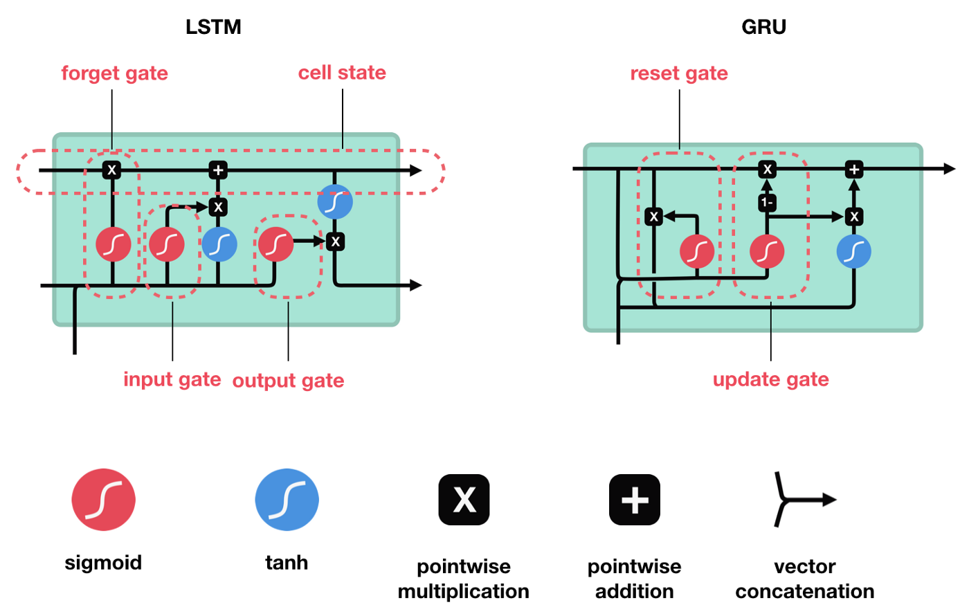
Let's break down the GRU's operations.

• Update Gate ($z_t$): This gate decides how much of the previous memory, $h_{t-1}$, to keep. It's analogous to a mix of LSTM's forget and input gates.

  $$z_t=\sigma (W_z[h_{t-1},x_t])$$

• Reset Gate ($r_t$): This gate determines how to combine the new input $x_t$ with the previous memory $h_{t-1}$. It decides how much of the past information to "forget" when creating the new candidate memory.

  $$r_t=\sigma (W_r[h_{t-1},x_t])$$

• Candidate Hidden State (${\tilde{h}}_t$): A new memory content is proposed, using the reset gate to selectively ignore parts of the previous state.

  $${\tilde{h}}_t=\tanh (W_h[r_t\odot h_{t-1},x_t])$$

• Final Hidden State ($h_t$): The update gate $z_t$ performs a linear interpolation between the old state $h_{t-1}$ and the new candidate state ${\tilde{h}}_t$.

  $$h_t=(1-z_t)\odot h_{t-1}+z_t\odot {\tilde{h}}_t$$

If the update gate $z_t$ is close to 0, the new state $h_t$ is almost identical to the old state $h_{t-1}$, allowing information and gradients to flow through easily.

The following video and article provide a concise explanation and the core formulas for the GRU.

In practice, there is no definitive winner between LSTM and GRU. LSTM's separate cell state may give it an edge in modeling particularly long and complex dependencies, but GRU's efficiency makes it a very strong contender, especially when computational resources are a concern.

Conclusion

This lesson moved from the problem of vanishing gradients in simple RNNs to the architectural solution provided by gating mechanisms. By introducing gates, LSTMs and GRUs gain dynamic, learned control over what information to remember and what to forget.

Key Takeaways:

• Gating Principle: LSTMs and GRUs use gates (small neural networks with sigmoid activations) to regulate the flow of information through the network.
• LSTM Architecture: Employs a separate cell state for long-term memory and controls it with a forget gate, an input gate, and an output gate.
• GRU Architecture: A simpler model that merges the cell and hidden states and uses just two gates: an update gate and a reset gate.
• The Gradient Highway: The crucial innovation in both architectures is the additive update mechanism (e.g., $c_t=f_t\odot c_{t-1}+...$). This creates a direct path for gradients to flow backward through time, conditioned by gate activations rather than being repeatedly multiplied by a fixed weight matrix. This allows the network to learn and preserve long-range dependencies.
• Practical Trade-offs: LSTMs are more expressive but computationally heavier. GRUs are faster and require fewer parameters, often performing on par with LSTMs.

Preview of the Next Lesson:

While LSTMs and GRUs were a monumental leap forward, they still process information sequentially, one step at a time. This can be a bottleneck for very long sequences and prevents parallelization during training. What if a model could look at all parts of a sequence simultaneously and decide which words are most important to each other, regardless of their distance? In our next lesson, we will introduce attention mechanisms, the foundation of the Transformer architecture, which does exactly that. We'll start by defining scaled dot-product attention as a powerful query-key-value lookup system.