The Degradation Problem in Deep Networks

Introduction

In our last lesson, we performed a detailed trace of the LeNet-5 architecture. We saw how a sequence of convolutional and pooling layers can systematically transform an image into a set of abstract features for classification. This established the foundational pattern of early CNNs: progressively decrease spatial dimensions while increasing feature depth. A natural question follows from this: if stacking a few layers is good, is stacking many more layers even better? Intuitively, more layers mean more parameters and greater representational power, which should lead to better performance.

This lesson confronts a surprising and counter-intuitive discovery that challenged this assumption. We will investigate the degradation problem, a phenomenon where making networks excessively deep actually increases the training error. We will first define the problem empirically, then explore why its existence presents a paradox for optimization theory. Finally, leveraging your interest in graphics and geometry, we will visualize the problem by examining how the loss landscape itself becomes pathologically non-convex and chaotic as depth increases, making it nearly impossible for optimizers like SGD to navigate.

Part 1: The Problem of Degradation

In the years following AlexNet's success, researchers pushed the boundaries of network depth. However, they soon hit a wall. Beyond a certain point, performance would not just saturate, but begin to rapidly degrade.

The seminal paper that addressed this, "Deep Residual Learning for Image Recognition," provides the clearest evidence. Let's look at the authors' own description of the problem.

To reinforce this core concept, the following video provides a concise summary of the problem.

After reviewing this material, you should have a clear empirical definition of the degradation problem: for "plain" deep networks (simple stacks of layers), at some point increasing depth leads to a higher training error.

Part 2: An Optimization Paradox

Your background in systems and engineering will appreciate the paradoxical nature of this problem. It is not a problem of representational capacity. A deeper network is strictly more powerful than a shallower one. This leads to a powerful Socratic question.

Socratic Question: Imagine you have a successfully trained, well-performing 20-layer network. Now, I give you a 56-layer network architecture. Is there a simple, constructive way to set the weights of this new, deeper network so that it performs at least as well as the 20-layer one?

This reveals the core paradox. A solution exists by construction that would allow the deeper model to perform at least as well as the shallower one. The fact that Stochastic Gradient Descent (SGD) not only fails to find this solution but actively converges to a worse one means the degradation problem is a failure of optimization. The optimizer is unable to traverse the parameter space to find this trivially good solution.

Let's see how the original authors and other experts frame this.

So, why is learning an identity mapping so hard for a stack of non-linear layers? A stack of CONV -> ReLU -> CONV -> ReLU layers does not have a natural inclination to learn the function $f(x)=x$. In fact, due to common weight initialization schemes (sampling from a zero-mean Gaussian) and regularization techniques like weight decay (which push weights towards zero), these layers have a stronger bias towards learning a zero function, $f(x)=0$. Learning the identity function is a non-trivial optimization task.

Part 3: A Geometric Perspective: The Chaotic Loss Landscape

This is where the problem becomes visually and geometrically intuitive, connecting directly to your interest in computer graphics. The failure of the optimizer can be understood by visualizing the shape of the loss function. A 2018 paper, "Visualizing the Loss Landscape of Neural Nets," provides a stunning illustration of what happens to this landscape as plain networks get deeper.

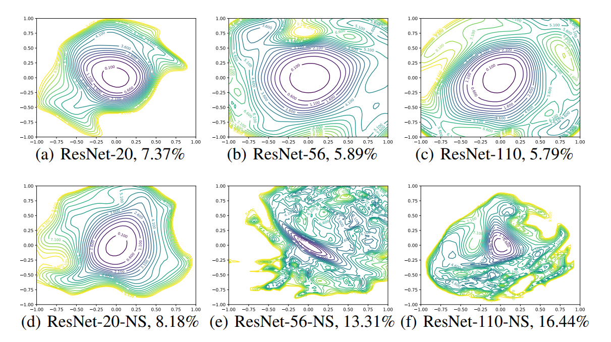
Let's analyze the bottom row, which represents the "plain" networks susceptible to degradation:

• (d) ResNet-20-NS (No-Shortcut): At 20 layers, the landscape is quite benign. It's dominated by a wide, seemingly convex basin. The contour lines are smooth and elliptical. For an optimizer like SGD, this is like rolling a ball down a smooth, wide bowl—it's easy to find the bottom.

• (e) ResNet-56-NS: At 56 layers, the landscape transforms dramatically. It becomes highly non-convex and "chaotic." While there is a minimum at the center, it's surrounded by bumpy, irregular terrain. The gradients (which are perpendicular to the contour lines) may no longer point reliably toward the minimum. The optimizer can easily get trapped in a local minimum or slowed down navigating this complex region.

• (f) ResNet-110-NS: At 110 layers, the situation is even worse. The central basin of attraction has become very narrow, and the surrounding landscape is extremely steep and chaotic. The authors note that the loss function becomes extremely large as we move away from the minimum. Training a network in such a landscape is exceptionally difficult.

This visualization provides a powerful geometric intuition for the degradation problem. The optimization fails because the underlying loss surface becomes pathologically non-convex and difficult to traverse for gradient-based methods.

The paper's authors describe this phenomenon in detail.

Conclusion

In this lesson, we have dissected the degradation problem from three different angles. We began with the empirical observation that simply making networks deeper can paradoxically lead to higher training error. We then understood this as a profound optimization paradox: even though a good solution is known to exist by construction (using identity mappings), SGD fails to find it. Finally, we developed a powerful geometric intuition, seeing how the loss landscape itself warps from a smooth bowl into a chaotic, treacherous terrain as network depth increases, trapping the optimizer.

Key Takeaways:

• Degradation Problem: Simply stacking more layers in a plain deep neural network can lead to higher training error beyond a certain depth. This is an optimization failure, not an overfitting issue.
• Optimization Paradox: A deeper network has the capacity to at least perform as well as a shallower one (by learning identity mappings for extra layers), but standard optimization algorithms fail to find this solution.
• Geometric Intuition: The degradation problem corresponds to the loss landscape becoming increasingly non-convex and "chaotic" with depth. This makes navigation for gradient-based optimizers extremely difficult, leading to convergence at poor solutions.

Preview of the Next Lesson:

Take one last look at the loss landscape visualization, but this time focus on the top row (a, b, c). Notice how, for these networks, the landscape remains wide, smooth, and well-behaved even at 110 layers. These are Residual Networks (ResNets). The architectural innovation that prevents the loss landscape from descending into chaos is the residual connection, also known as a skip connection. In our next lesson, we will dive back into the original ResNet paper to understand the mechanics of these connections and how they elegantly solve the degradation problem.