LeNet-5: Architecture and Tensor Flow

Introduction

In our last lesson, we explored the fascinating emergent property of feature hierarchies in CNNs. We saw how stacking simple convolutional layers allows a network to learn representations of increasing complexity, from edges and colors to object parts and entire objects. We also established the crucial role of the receptive field in this process.

Now, it's time to ground these abstract concepts in a concrete, historical example. This lesson moves from the what and why to the how, by dissecting one of the most influential early CNNs: LeNet-5. Proposed by Yann LeCun et al. in 1998, this architecture was a trailblazer for document recognition and laid the groundwork for modern deep learning in computer vision. We will perform a systematic, layer-by-layer trace of the data flow, calculating the shape of the data tensors at each step. This process is akin to tracing signals through a circuit or data through a low-level system, allowing us to build a first-principles understanding of an end-to-end vision network.

Part 1: The Mathematics of Tensor Shapes

Before we start our dissection of LeNet-5, we must have our primary tool ready: the formula for calculating the output dimensions of a convolutional or pooling layer. In the previous lesson, we focused on the receptive field, which looks backward from an output neuron to the input. Now, we will look forward to determine the shape of the output volume.

The key insight is that the spatial dimensions (width and height) and the depth (channels) of the output are calculated differently.

With this mathematical framework, we are now equipped to trace any CNN architecture.

Part 2: Dissecting LeNet-5

We will now walk through the LeNet-5 architecture layer by layer. For each step, we'll note the input shape, the layer's parameters, and use our formula to calculate the output shape.

The following video provides an excellent visual walkthrough of this exact process. We will use it as our guide.

Layer 0: Input

The input to LeNet-5 is a 32x32x1 single-channel (grayscale) image. The original MNIST digits are 28x28, but they were placed in a 32x32 canvas. This padding ensures that features like corners and stroke endpoints, which might be at the edge of the 28x28 box, can fall into the center of a kernel's receptive field in the first layer.

---

Layer C1: First Convolutional Layer

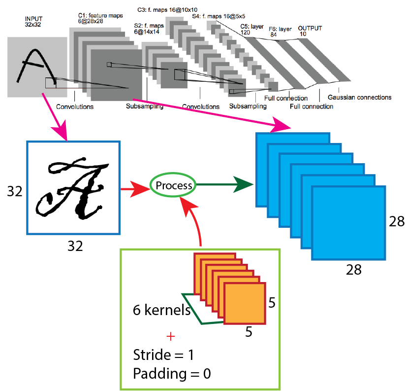
• Input Shape: 32x32x1
• Operation: Convolution
• Parameters:
  • Number of filters ($n_k$): 6
  • Kernel size ($k$): 5x5
  • Stride ($s$): 1
  • Padding ($p$): 0
• Calculation:
  • Spatial Dimensions: Using our formula, the output width and height are:
    $W_{out}=H_{out}=\lfloor \frac{32-5+2(0)}{1}\rfloor +1=27+1=28$
  • Depth: The output depth is equal to the number of filters.
    $D_{out}=6$
• Output Shape: 28x28x6

You can verify this by watching the corresponding segment in the video guide.

---

Layer S2: First Subsampling (Pooling) Layer

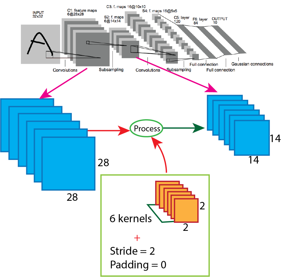
• Input Shape: 28x28x6
• Operation: Subsampling (Average Pooling). Modern architectures typically use Max Pooling.
• Parameters:
  • Kernel size ($k$): 2x2
  • Stride ($s$): 2
  • Padding ($p$): 0
• Calculation:
  • Spatial Dimensions:
    $W_{out}=H_{out}=\lfloor \frac{28-2+2(0)}{2}\rfloor +1=13+1=14$
  • Depth: Pooling operates on each channel independently, so the depth remains unchanged.
    $D_{out}=6$
• Output Shape: 14x14x6

The video guide confirms this calculation.

---

Layer C3: Second Convolutional Layer

• Input Shape: 14x14x6
• Operation: Convolution
• Parameters:
  • Number of filters ($n_k$): 16
  • Kernel size ($k$): 5x5
  • Stride ($s$): 1
  • Padding ($p$): 0
• Calculation:
  • Spatial Dimensions:
    $W_{out}=H_{out}=\lfloor \frac{14-5+2(0)}{1}\rfloor +1=9+1=10$
  • Depth: The output depth is the number of new filters.
    $D_{out}=16$
• Output Shape: 10x10x16

A Note on Connectivity: In the original 1998 paper, this layer used a complex, sparse connection scheme to reduce parameters and break symmetry. Not all 16 output feature maps were connected to all 6 input feature maps. Modern implementations, optimized for GPUs, typically ignore this and use a standard "fully connected" convolution where each of the 16 filters has a depth of 6 and is convolved across all input channels.

You can watch the video explanation for this layer.

---

Layer S4: Second Subsampling (Pooling) Layer

• Input Shape: 10x10x16
• Operation: Subsampling (Average Pooling)
• Parameters:
  • Kernel size ($k$): 2x2
  • Stride ($s$): 2
  • Padding ($p$): 0
• Calculation:
  • Spatial Dimensions:
    $W_{out}=H_{out}=\lfloor \frac{10-2+2(0)}{2}\rfloor +1=4+1=5$
  • Depth: Unchanged.
    $D_{out}=16$
• Output Shape: 5x5x16

This is the final output of the convolutional "backbone" of LeNet-5. At this point, the network has transformed the 32x32 image into 16 abstract feature maps, each of size 5x5.

---

Layers C5, F6, and Output: The Classifier Head

After feature extraction, the network must perform classification. This is handled by a series of layers that transition from 3D tensors to a final 1D vector of class probabilities.

1. Layer C5 (Convolution as a Fully Connected Layer):

   • Input Shape: 5x5x16
   • Operation: Convolution
   • Parameters: 120 filters, 5x5 kernel, stride 1, padding 0.
   • Output Shape: Let's calculate: $W_{out}=(5-5+0)/1+1=1$. The output is 1x1x120.
   • Interpretation: A convolution with a kernel size equal to the input size results in a 1x1 output for each filter. This is functionally equivalent to flattening the 5x5x16 input into a vector of length 400 ($5\times 5\times 16$) and applying a fully connected layer with 120 output neurons.

2. Flattening: The 1x1x120 tensor is flattened into a vector of 120 elements.

3. Layer F6 (Fully Connected Layer):

   • Input: 120 neurons
   • Operation: Fully Connected (matrix multiplication + bias)
   • Output: 84 neurons. This number was chosen for a historical reason related to the bitmap representation of characters on a terminal.

4. Output Layer (Fully Connected Layer):

   • Input: 84 neurons
   • Operation: Fully Connected
   • Output: 10 neurons, one for each digit class (0-9).
   • Activation: A softmax function is applied to these 10 outputs to convert them into a probability distribution.

The video guide concludes with an explanation of these final layers.

The GeeksForGeeks article LINK also provides a concise table summarizing the entire architecture, which is a great reference.

Part 3: Parameter Efficiency

Your systems background will appreciate the importance of efficiency. One of the primary motivations for convolution is parameter sharing, which dramatically reduces the number of trainable weights compared to using fully connected layers on images. Let's quantify this.

Socratic Question:

1. Consider layer C3, which takes a 14x14x6 input and produces a 10x10x16 output using 5x5 kernels. Assuming a modern implementation (each output channel connects to all input channels), calculate the total number of trainable parameters (weights + biases) for this layer.
2. Now, imagine you tried to achieve a similar mapping using only a fully connected layer. It would take an input vector of size $14\times 14\times 6=1176$ and produce an output vector of size $10\times 10\times 16=1600$. How many trainable parameters would this FC layer require?
3. What does the enormous difference in these two numbers tell you about the fundamental operating principle of convolutional layers?

Answer

1. **Convolutional Layer (C3) Parameters:** * Each of the 16 filters has a shape of $5 \times 5 \times 6$ (kernel width x kernel height x input depth). * Number of weights per filter: $5 \times 5 \times 6 = 150$. * Each filter also has 1 bias term. So, $150 + 1 = 151$ parameters per filter. * Total parameters for 16 filters: $151 \times 16 = \mathbf{2,416}$.

2. Fully Connected Layer Parameters:

   • Input neurons: $14\times 14\times 6=1176$.
   • Output neurons: $10\times 10\times 16=1600$.
   • Number of weights: $1176\times 1600=1,881,600$.
   • Number of biases: $1600$.
   • Total parameters: $1,881,600+1,600=1,883,200$.

3. Conclusion: The convolutional layer requires almost 800 times fewer parameters to perform a similar input-output mapping. This staggering efficiency comes from two principles:

   • Parameter Sharing: The same $5\times 5\times 6$ filter is reused (slid across) all spatial locations of the input. An FC layer, in contrast, learns a unique weight for every single input-output neuron connection.
   • Locality: A convolutional layer assumes that features are local. An output neuron is only affected by its local receptive field, not by pixels on the other side of the image. An FC layer breaks this assumption, connecting every output to every input.

Conclusion

By tracing LeNet-5, we have solidified our understanding of how the core components of a CNN—convolution, padding, stride, and pooling—work together in a complete system. We have seen firsthand how an architecture progressively reduces spatial dimensions while increasing feature depth, transforming a grid of pixels into a set of abstract, class-relevant features.

Key Takeaways:

• Architectural Pattern: LeNet-5 established the classic CNN pattern of stacking convolutional and pooling layers to extract features, followed by fully connected layers for classification.
• Tensor Shape Calculation: The shape of tensors changes predictably at each layer, governed by simple mathematical formulas relating input size, kernel size, stride, and padding.
• Dimensionality Trade-off: CNNs typically decrease height and width while increasing the number of channels (depth). This transforms low-level spatial information into high-level feature information.
• Parameter Efficiency: The use of parameter sharing in convolutional layers offers a monumental reduction in model size compared to using fully connected layers on raw pixels.

Preview of the Next Lesson:

While LeNet-5 was revolutionary, as networks grew deeper, a new problem emerged: the degradation problem, where adding more layers actually hurt performance. In our next lesson, we will investigate why this happens and explore the simple yet profound architectural innovation that solved it: residual connections, as introduced in the groundbreaking ResNet architecture.