Recommended resources
The freely available resources this lesson will direct you to.
Introduction
In our last lesson, we delved into the low-level mechanics of a single convolutional layer, implementing its forward and backward passes from first principles. We now possess a granular understanding of how filters extract features and how their weights are updated via backpropagation. It's time to zoom out and discover what happens when we stack these layers one after another.
This lesson explores one of the most profound and powerful emergent properties of deep learning: the feature hierarchy. We will investigate how a Convolutional Neural Network, through the simple act of stacking layers, learns to represent the world in a way that mirrors our own visual processing—starting with simple patterns and composing them into increasingly abstract and meaningful concepts. We'll examine the seminal visualization techniques that first revealed this internal world and dissect the core mechanisms, particularly the concept of the receptive field, that make this hierarchical learning possible.
Part 1: Visualizing What CNNs Learn
The question of what goes on inside a trained neural network—often dubbed the "black box" problem—was a major focus of early deep learning research. A groundbreaking 2013 paper by Matthew Zeiler and Rob Fergus, "Visualizing and Understanding Convolutional Networks," provided one of the first clear windows into the inner workings of a CNN. They developed a technique using a "deconvolutional network" to project the features learned by filters back into the input pixel space, allowing us to see what kind of patterns maximally activate a given neuron.
The results revealed a stunning hierarchy of feature complexity. Let's watch a presentation by one of the authors, Matt Zeiler, where he walks through the features learned at each layer of their trained network.
Visualizing and Understanding Deep Neural Networks by Matt Zeiler
This video, presented by the author of the seminal paper on CNN visualization, provides a direct tour of the feature hierarchy.
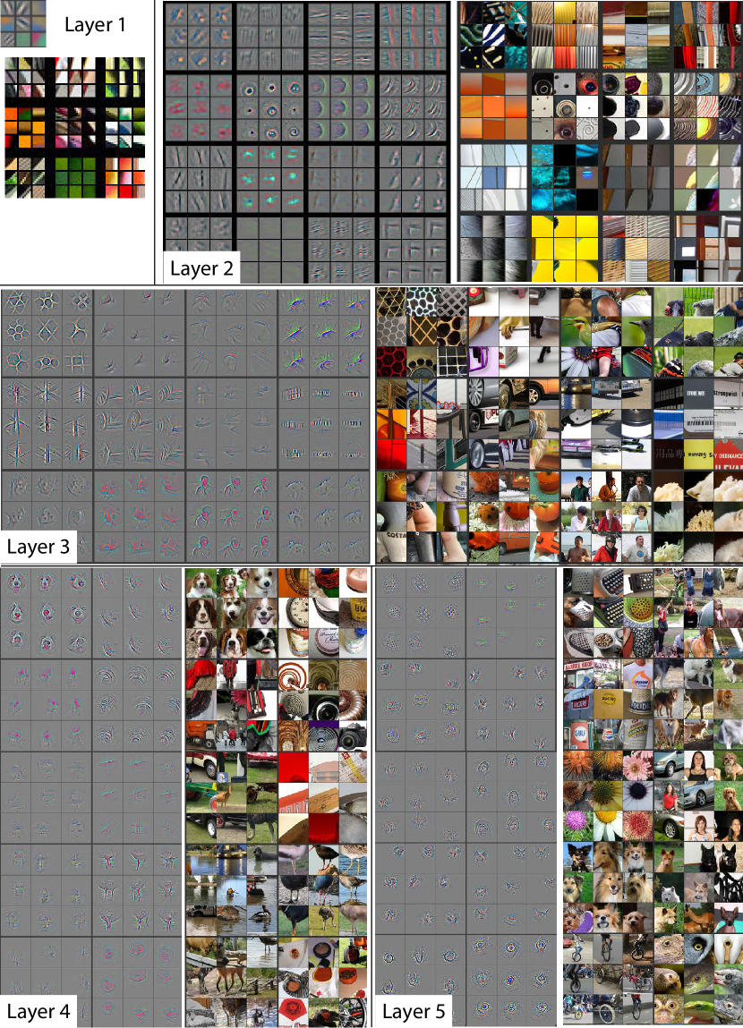
First, watch the brief overview of a CNN architecture from this segment to refresh the concepts. Next, observe the visualizations for each layer sequentially. Pay close attention to the description of what is being learned: Layer 1: Simple edges and colors. Layer 2: Combinations of edges forming corners, textures, and simple patterns. Layer 3: More complex object parts like faces, eyeballs, and specific textures (e.g., honeycombs, clouds). Layer 4: More complete object parts and class-specific features, like dog faces. Layer 5: Highly specific, almost full-object representations, such as keyboards, water, and even specific dog breeds.
The image below, taken directly from the Zeiler and Fergus paper, summarizes these findings. On the left of each layer's section, you see the visualized features (the patterns the filters look for). On the right, you see the patches from actual images in the dataset that caused the highest activation for those features.
To round out your understanding of visualization techniques, the following video provides a concise overview of different methods, including the deconvolutional approach we've just seen and an alternative optimization-based method that generates a synthetic image from scratch to activate a neuron.
'How neural networks learn' - Part I: Feature Visualization
This Arxiv Insights video explains several methods for visualizing what neural networks learn.
Watch the segments on dataset example visualization, deconvolution, and optimization-based visualization. This will give you a broader toolkit for thinking about network interpretability. The final summary at the recap nicely encapsulates the core idea of hierarchical feature learning.
Part 2: The Mechanisms of Hierarchical Learning
Now that we've seen what happens, we need to understand why it happens. This hierarchical learning is not an explicitly programmed behavior; it's an emergent property that arises from two fundamental mechanisms: compositionality and an expanding receptive field.
1. Compositionality
The principle of compositionality is straightforward: each layer in a CNN takes the output feature maps of the previous layer as its input.
- Layer 1 filters operate on raw pixels to detect simple patterns (e.g., a horizontal edge).
- Layer 2 filters operate on the feature maps from Layer 1. A filter in Layer 2 might learn to activate when it sees the output of a "horizontal edge" detector next to the output of a "vertical edge" detector. In doing so, it has effectively learned a "corner" detector.
- Layer 3 filters can then combine corner detectors, curve detectors, and texture detectors from Layer 2 to form more complex parts, like an "eye" detector.
This process continues, with each layer building more complex representations from the slightly simpler concepts learned by the layer before it.
2. The Receptive Field
For a layer to combine features into something larger (like combining wheel, window, and headlight features into a car), its neurons must be able to "see" a sufficiently large region of the original input image. This brings us to the critical concept of the receptive field.
The receptive field of a neuron in a convolutional network is the specific region of the input image that affects that neuron's activation.
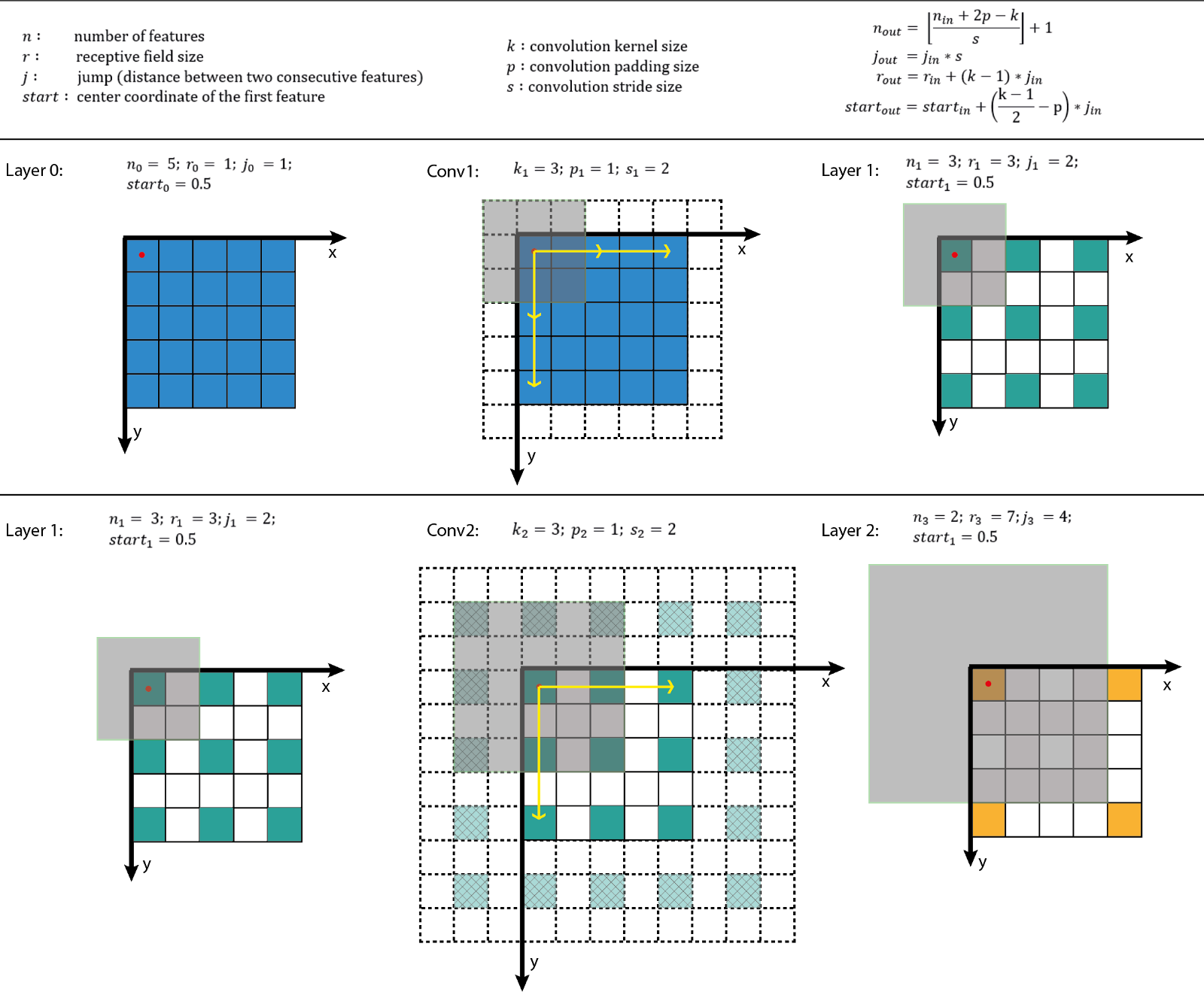
A neuron in the first convolutional layer has a receptive field equal to the kernel size (e.g., 3x3 or 5x5). However, a neuron in the second layer, which looks at a 3x3 patch of the first layer's feature map, is indirectly influenced by a larger region of the original input. This is because each of the neurons in that 3x3 patch it's looking at had its own receptive field in the input image.
The following resource provides an excellent, in-depth guide to understanding and calculating receptive fields.
Receptive Field: Understanding CNN Vision
This article explains the concept, mathematics, and architectural impact of receptive fields.
Start by reading the sections "What is a Receptive Field?" to get a solid conceptual grounding. This directly connects the receptive field to the feature hierarchy. Next, study the "Mathematical Formulation" section. Given your systems background, you will appreciate the precise formulas for calculating how the receptive field size r and jump j (total stride) grow layer by layer. Finally, read the section "Architecture Impact". This explains how standard convolutions, and especially pooling or strided convolutions, contribute to receptive field growth.
Socratic Question: Imagine you are designing a CNN for two different tasks:
- Detecting small, cancerous cells (e.g., 20x20 pixels) in a very large medical image (e.g., 4000x4000 pixels).
- Classifying the overall scene of a landscape photograph (e.g., 'beach' vs. 'forest').
How might you want the receptive field of the final feature-extracting layers to differ between these two networks, and why? What architectural choices could you make to achieve this?
Answer
* For **Task 1 (small object detection)**, you would want the receptive field of the feature detectors to be relatively small, perhaps only slightly larger than the objects of interest (e.g., 30x30 to 60x60 pixels). A massive receptive field (e.g., 1000x1000) would wash out the fine-grained information of the small cancer cell with context from a large, mostly irrelevant background. The network would struggle to localize and identify the small object. To achieve this, you might design a network that is deep but uses very little or no pooling/striding, relying on many stacked 3x3 convolutions to slowly grow the receptive field.- For Task 2 (scene classification), you need to integrate information from across the entire image. Therefore, you would want the receptive field of the final feature layers to be very large, ideally covering the entire input image. This allows the network to combine features like "sand," "water," and "blue sky" to conclude the scene is a "beach." To achieve this, you would use a standard CNN architecture with multiple pooling or strided convolution layers, which aggressively increase the receptive field at the expense of spatial resolution (which is less critical for whole-image classification).
Part 3: From Hierarchical Features to Classification
The feature hierarchy is built by the convolutional "backbone" of the network. But how does this lead to a final classification?
The output of the final convolutional layer is a set of feature maps that represent the most abstract concepts the network has learned. For an image of a dog, these feature maps might have high activations in regions corresponding to "snout," "floppy ears," and "furry texture."
These 3D tensors of feature maps are then flattened into a single long vector. This vector serves as the input to a standard fully connected classifier (the "head" of the network), just like the MLPs we've discussed previously. This classifier's job is to learn which combinations of these abstract features correspond to which classes.
Convolutional Neural Network (CNN): A Complete Guide
This section explains how the features from the convolutional backbone are used by the classifier head.
Read the sections "Fully Connected Classifier" and "Intuition for Why CNNs Work". Focus on how the network maps the spatial features from the convolutional layers to a final class probability.
The fully connected layers can weigh the importance of features from all spatial locations. If the "dog snout" feature is active in the center, a "dog ear" feature is active in the upper-left, and a "tail" feature is active on the right, the trained weights in the fully connected layers will combine these signals to produce a high output for the "dog" class neuron.
Conclusion
In this lesson, we have moved from the single-layer mechanics of convolution to the architectural-level understanding of how CNNs function. We've seen that by stacking layers, a network autonomously learns a rich, hierarchical set of features that progresses from simple to complex.
Key Takeaways:
- Hierarchical Feature Learning: CNNs learn features in a compositional hierarchy. Early layers detect simple primitives like edges and colors, while deeper layers combine these to form textures, object parts, and eventually, full object representations.
- Visualization: Techniques like deconvolution allow us to visualize the patterns that specific filters learn, providing a window into the network's "mind."
- Receptive Field: The receptive field of a neuron determines the size of the input region it can "see." It grows with network depth, especially through the use of pooling or strided convolutions, enabling neurons in deeper layers to learn about larger, more complex structures.
- Backbone and Head: A typical CNN is composed of a convolutional "backbone" that acts as a hierarchical feature extractor, followed by a fully connected "head" that acts as a classifier, mapping the extracted features to class probabilities.
Preview of the Next Lesson:
Now that we understand the individual components (convolution, pooling) and the emergent property of feature hierarchies, we are ready to analyze a complete, end-to-end architecture. In the next lesson, we will dissect one of the pioneering CNNs, LeNet-5. We will trace the flow of data through its layers, calculating the shape of the tensors at each stage and solidifying our understanding of how these parts work together to solve a real-world image classification problem.