2D Convolution: Forward and Backward Pass from Scratch

Introduction

In our previous lessons, we've built a conceptual framework for Convolutional Neural Networks, understanding the roles of convolutional filters for feature extraction and pooling layers for creating spatial invariance. We now arrive at a pivotal moment in your journey from theory to practice: implementing the complete forward and backward pass for a 2D convolution layer from scratch. This is the heart of any CNN and a non-trivial engineering challenge.

This lesson will connect directly with your interest in high-performance systems. We will not only implement the operations but also analyze how they are implemented efficiently in real-world libraries. You will see how a series of nested loops can be transformed into a single, highly optimized matrix multiplication—a classic trick of the trade. We will then apply our mastery of multivariable calculus to derive the backpropagation equations, seeing how the gradients themselves take the form of convolutions.

By the end of this lesson, you will have derived and implemented the most computationally demanding component of a modern vision model.

Part 1: The Forward Pass - From Naive Loops to Optimized Matrix Multiplication

The forward pass of a convolution layer is defined by the cross-correlation operation. The most direct way to implement this is with a set of nested loops that slide the kernel over the input tensor, computing the dot product at each position.

The resource "Build a Simple Deep Learning Library" provides a clear, if highly inefficient, implementation of this idea.

Seeing eight nested loops should immediately raise a red flag from a performance standpoint. Such an implementation suffers from poor memory locality and fails to leverage the highly optimized, parallel matrix multiplication routines available in modern CPUs and GPUs (e.g., BLAS, cuBLAS).

This leads to a critical question for any systems-oriented engineer: how can we re-frame this operation to be faster?

Question: We can implement convolution with nested loops or by transforming it into a single, large matrix multiplication (a technique called im2col). From a systems perspective, what are the trade-offs between these two approaches? Think about memory access patterns, cache utilization, and the ability to leverage existing optimized libraries.

Answer

The nested loop approach, while intuitive, is a performance disaster. It involves many small, non-contiguous memory accesses as it picks out elements from the input tensor. This leads to frequent cache misses and prevents effective vectorization (SIMD instructions).

The im2col ("image-to-column") approach transforms the problem entirely. It involves an initial, potentially costly, memory reorganization step where overlapping patches of the input image are laid out as columns in a new, large matrix. The kernel is also reshaped into a row vector. After this setup, the entire convolution operation becomes a single, large matrix-matrix multiplication (GEMM - General Matrix Multiply).

The trade-offs are:

• Memory: im2col uses significantly more memory because it explicitly duplicates the data from overlapping patches.
• Performance: Despite the memory overhead, im2col is vastly faster. It allows us to use highly-optimized BLAS libraries (like OpenBLAS, MKL, cuBLAS) that are the product of decades of research. These libraries feature near-perfect cache utilization, vectorization, and parallelism, making the GEMM operation orders of magnitude faster than the naive loop implementation. For deep learning, this performance gain is non-negotiable.

Let's now study the im2col trick in detail. The same resource provides an excellent explanation, culminating in a highly efficient implementation that uses a clever NumPy function, as_strided, to create the column matrix without actually duplicating memory. This is a low-level memory view manipulation that should appeal to your systems programming interests.

Part 2: The Backward Pass - The Mathematics of Gradient Flow

Now we turn to the more complex task: backpropagation. Our goal is to compute three gradients:

1. Gradient with respect to the weights ($\frac{\partial E}{\partial W}$): To update the kernel.
2. Gradient with respect to the input ($\frac{\partial E}{\partial A}$): To propagate the error to the previous layer.
3. Gradient with respect to the bias ($\frac{\partial E}{\partial b}$): To update the bias term.

To begin, we must be precise about our terminology. In deep learning, the "convolution" in the forward pass is almost always implemented as cross-correlation. A true mathematical convolution requires flipping the kernel by 180 degrees. This distinction becomes critical during backpropagation.

This short video segment clarifies the difference.

With that distinction in mind, let's derive the gradients.

Gradient w.r.t. Weights ($\frac{\partial E}{\partial W}$)

Consider a single weight $W_{ij}$ in the kernel. As the kernel slides across the input, this weight multiplies different input activations $A_{uv}$. The total gradient for $W_{ij}$ is the sum of its contributions to the final error $E$, chained through every output pixel $Z_{xy}$ it affects.

It turns out this complex summation can be expressed elegantly as another convolution. The gradient with respect to the weights is the convolution of the input activation tensor $A$ with the output gradient tensor ${\delta }^{(l)}=\frac{\partial E}{\partial Z^{(l)}}$.

$$\frac{\partial E}{\partial W^{(l)}}=A^{(l-1)}\otimes {\delta }^{(l)}$$

Here, $\otimes$ denotes a 'valid' convolution. To see the full derivation, let's turn to a more formal mathematical resource.

The video resource provides a more visual derivation of the same result.

Gradient w.r.t. Input ($\frac{\partial E}{\partial A}$)

Propagating the gradient to the previous layer ($\frac{\partial E}{\partial A^{(l-1)}}$) is essential for training deep networks. The derivation is analogous but reveals a fascinating symmetry. This operation is equivalent to convolving the output gradient ${\delta }^{(l)}$ with the 180-degree rotated kernel $W^{(l)}$.

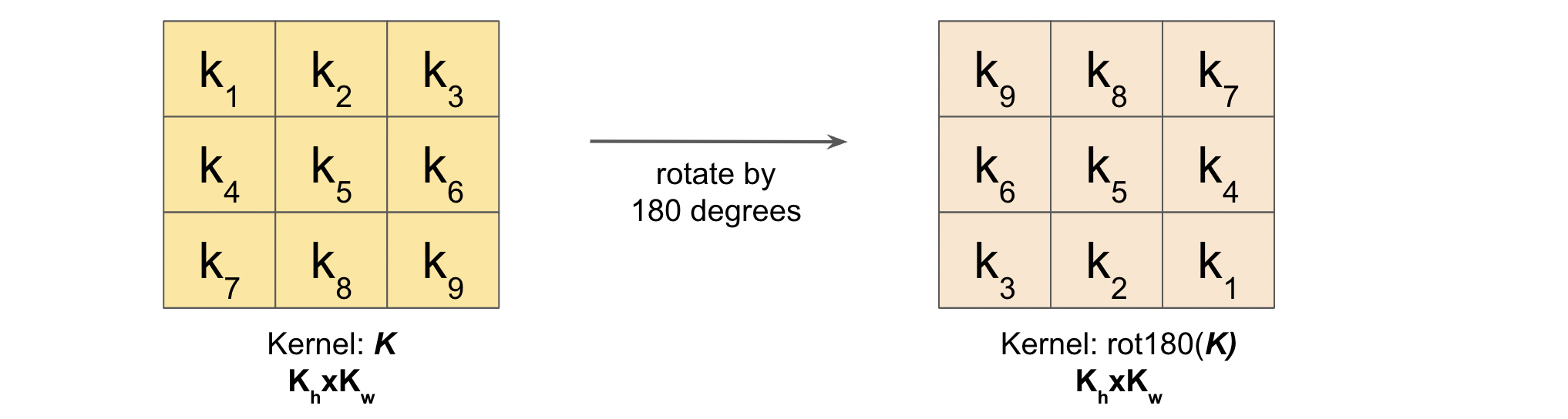
Furthermore, to ensure the resulting gradient tensor $\frac{\partial E}{\partial A^{(l-1)}}$ has the same spatial dimensions as the original input $A^{(l-1)}$, this operation must be a "full" convolution, which involves padding the input (${\delta }^{(l)}$) such that the output dimensions are expanded.

The final equation is:

$$\frac{\partial E}{\partial A^{(l-1)}}={\delta }^{(l)}{\otimes }_{full}\text{rot180}(W^{(l)})$$

Let's see the derivation in our text and video resources.

Gradient w.r.t. Bias ($\frac{\partial E}{\partial b}$)

The bias gradient is the most straightforward. Since the bias $b_k$ for a given filter $k$ is added to every element of the corresponding output feature map $Z_k$, its gradient is simply the sum of all elements in the output gradient map ${\delta }_k$.

$$\frac{\partial E}{\partial b_k^{(l)}}=\sum _{i,j}({\delta }_k^{(l)}{)}_{ij}$$

The video from "The Independent Code" walks through this simple derivation.

Part 3: From-Scratch Implementation of the Backward Pass

Now, let's translate these mathematical formulas into Python code. The video "Convolutional Neural Network from Scratch" provides a complete implementation of the backward method, using scipy.signal which has separate functions for correlate (for the forward pass and weight gradient) and convolve (for the input gradient).

For a more advanced implementation that correctly handles stride > 1 (which requires "dilating" the output gradient), the "Build a Simple Deep Learning Library" resource is an excellent next step for independent exploration. It shows how to build flip and dilate operations to construct a fully general backward pass. This is precisely how high-performance libraries are built. You can explore section 10.8 Conv Backward in that resource (LINK) on your own.

Conclusion

In this lesson, we have plunged into the mechanical core of the convolutional layer. We've gone from a high-level understanding to a first-principles implementation of both the forward and backward passes.

Key Takeaways:

• Forward Pass Optimization: The forward pass, a cross-correlation, can be transformed from a slow, loop-based algorithm into a highly efficient matrix multiplication using the im2col technique.
• Backward Pass as Convolutions: Backpropagation through a convolutional layer is not matrix multiplication but rather a series of convolution operations.
  • The weight gradient ($\frac{\partial E}{\partial W}$) is a valid convolution between the input activations and the output gradient.
  • The input gradient ($\frac{\partial E}{\partial A}$) is a full convolution between the output gradient and the 180-degree rotated kernel.
• Symmetry of Operations: There is a beautiful symmetry where the forward pass is a cross-correlation, and the backward passes are true convolutions, highlighting the deep mathematical structure underlying neural networks.

Preview of the Next Lesson:

With the low-level mechanics of the convolutional layer now firmly in hand, we can zoom back out to the architectural level. In our next lesson, we will explore how stacking these layers creates a feature hierarchy, where the network learns progressively more abstract and complex features—from simple edges and colors in the early layers to object parts and entire objects in the deeper layers. This is the emergent property that gives CNNs their remarkable power in computer vision.