Recommended resources
The freely available resources this lesson will direct you to.
Introduction
In our last lesson, we formalized the convolutional layer, exploring how filters, stride, and padding give us precise control over feature extraction and the spatial dimensions of our data. We saw that using a stride greater than one is a direct way to downsample feature maps, reducing their size. This lesson introduces another fundamental operation in CNN architectures that accomplishes a similar goal but with a different mechanism and purpose: the pooling layer.
We will explore the two primary types of pooling—max pooling and average pooling—and unpack their dual roles within a network. You will learn how these simple, deterministic operations are critical for managing computational complexity and, most importantly, for building spatial invariance into the model, allowing it to recognize features regardless of their exact position. This concept is a cornerstone of robust object recognition.
What is a Pooling Layer?
At its core, a pooling layer performs a downsampling operation, reducing the spatial dimensions (width and height) of a feature map. Unlike a convolutional layer, which uses learnable kernels, a pooling layer applies a fixed, deterministic function to regions of the input. It slides a window—typically 2x2—across the feature map and aggregates the values within that window into a single output value.
The two most common aggregation functions define the two main types of pooling:
- Max Pooling: Takes the maximum value from each window.
- Average Pooling: Takes the average value from each window.
To see this in action, consider the following activation map.
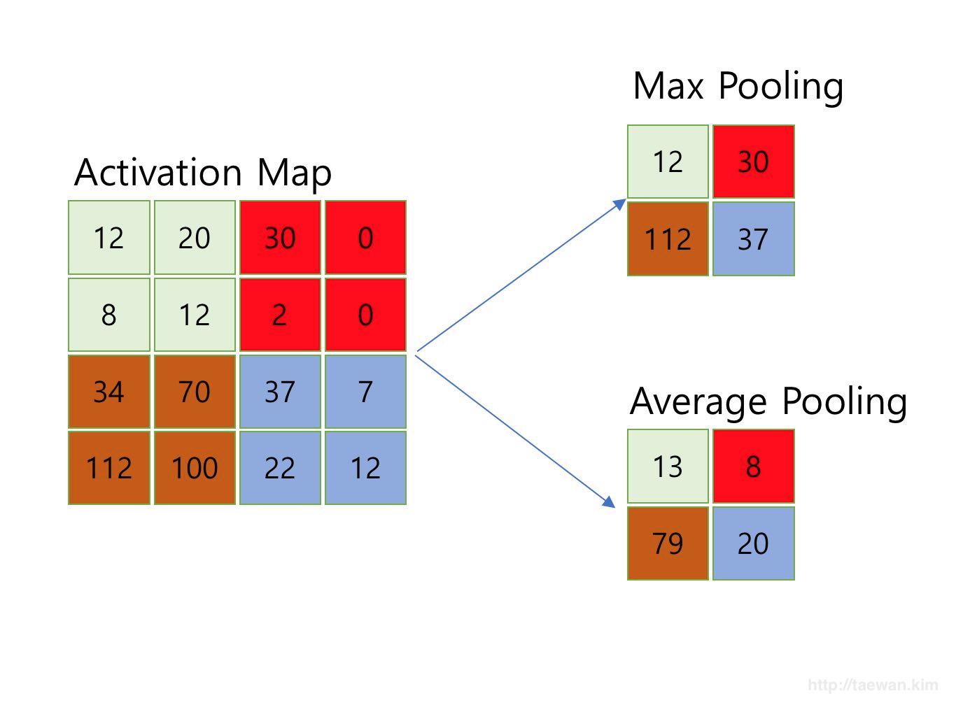
Notice a crucial difference from the convolutional layers we've studied: there are no weights or biases to learn. The operation is a fixed function. This makes pooling computationally inexpensive and a powerful tool for the network architect.
To formalize this, please read the following brief introductions from two excellent resources. The first, from Stanford's CS231n course, defines the layer's mechanics. The second, from Dive into Deep Learning, provides context and a clear diagram.
https://cs231n.github.io/convolutional-networks/
This section from the CS231n notes provides a technical summary of the pooling layer.
Read the section titled "Pooling Layer". Pay close attention to the list of hyperparameters (F and S) and the fact that pooling layers introduce zero parameters.
7.5. Pooling — Dive into Deep Learning 1.0.3 documentation
This text introduces the motivation and mechanics of pooling operations.
Read the section "Maximum Pooling and Average Pooling". This will solidify the definition of both max and average pooling with a clear diagram and example calculation.
The Dual Purpose of Pooling
Now that we understand what pooling is, the critical question is why we use it. While downsampling is the immediate effect, it serves two strategic purposes in a deep network.
1. Dimensionality Reduction and Computational Efficiency
This first purpose will appeal to your interest in high-performance systems. As a network gets deeper, we typically increase the number of channels (i.e., the number of filters in each convolutional layer) to learn increasingly complex and abstract features. If we kept the spatial dimensions the same, the total number of activations, and thus the computational and memory requirements, would explode.
Pooling provides an effective way to manage this complexity. By periodically reducing the width and height of the feature maps, we can afford to increase their depth (number of channels) without overwhelming our computational budget.
This video provides a great visualization of this trade-off.
What are Pooling Layers in Deep Neural Networks?
This video by Deep Learning with Yacine clearly explains the role of pooling in managing network complexity.
Watch the segment from dimensionality reduction. Notice the inverse relationship the speaker describes: as the network gets deeper, the number of filters increases while the spatial dimensions decrease, keeping the total "volume of information" in check.
2. Creating Spatial Invariance
This is arguably the more profound contribution of pooling layers. In the previous lesson, we discussed that convolution is translationally equivariant: shifting the input object shifts the resulting feature map. While useful, for tasks like image classification, we ultimately want invariance: the classifier's final output should not change if the object moves slightly. We want to detect a cat whether it's in the top-left or center of the image.
Max pooling, in particular, helps build this invariance at a local level. By taking the maximum value in a region, the network becomes less sensitive to the exact location of the feature. All that matters is that the feature was strongly detected somewhere within that pooling window.
The following image provides a perfect illustration of this principle.

This property means the network can learn to recognize a feature without having to learn a separate detector for every possible small shift.
To deepen your understanding of this key concept, the following video clips provide excellent explanations.
What are Pooling Layers in Deep Neural Networks?
This section of the video explicitly tackles the concept of translational invariance.
Watch the segment from translational invariance. The speaker does a great job of distinguishing invariance (output doesn't change) from the equivariance provided by convolution.
Equivariant Neural Networks Part 13 - Introduction
This clip from DeepFindr provides a concise and formal definition of invariance.
Watch from invariance. The idea of pooling as a "set function" (like max or mean) that is inherently invariant to the order or position of elements within the set is a powerful mental model.
With these concepts in mind, here is a question for you to consider:
We've established that max pooling creates local translation invariance by selecting the most prominent feature in a region. Average pooling, on the other hand, considers all activations in the window. What trade-off do you think we are making when choosing max pooling over average pooling, especially when considering images with fine-grained textures versus images with large, distinct objects?
Answer
When we choose max pooling, we are making a bet that the most important information in a local region is the *presence* of a strong feature. This makes it very effective for detecting the corners, edges, and parts of distinct objects, as it preserves the strongest signals while discarding weaker, potentially noisy activations. The trade-off is that it throws away a significant amount of information about the texture and overall composition of the region.Average pooling, by contrast, preserves more of the "background" information. It tells us about the average feature response in a region. This can be a disadvantage, as it can dilute a single, strong feature signal, making the network less decisive. This is why max pooling has been shown to perform better in practice for most computer vision tasks like object recognition. Average pooling might be slightly more suitable for tasks where preserving smooth, textural information is more critical than identifying sharp features, but it is far less common in modern architectures.
From-Scratch Implementation
To solidify your understanding from a first-principles perspective, let's look at how a pooling layer is implemented. The logic is a straightforward extension of the sliding-window concept from convolution.
The resource Dive into Deep Learning provides a clean, from-scratch implementation in Python that perfectly illustrates the mechanics.
7.5. Pooling — Dive into Deep Learning 1.0.3 documentation
This resource provides a from-scratch Python implementation of a 2D pooling function.
Focus on the Python code block starting with the function definition <span data-type="resource_reading_textrange" data-resource-subitem-id="627130a7" data-range-start="def pool2d(X, pool_size, mode = 'max'):" data-range-end="return Y">pool2d</span>. Analyze how it iterates over the dimensions of the output tensor Y and, for each (i, j) position, selects a window from the input X to apply either the .max() or .mean() operation. You'll see this logic is much simpler than the cross-correlation we saw for convolution.
This implementation clearly shows the deterministic nature of the pooling operation. Given an input X and a configuration (pool_size, mode), the output is always the same, with no learning involved.
Conclusion
In this lesson, we have dissected the pooling layer, a simple yet powerful component of nearly all classical CNN architectures. It complements the convolutional layer by providing a mechanism for downsampling and building robustness into the network's feature detectors.
Key Takeaways:
- Pooling Layers perform downsampling using a fixed, deterministic operation (like
maxoraverage) within a sliding window. They have no learnable parameters. - Dimensionality Reduction: Pooling reduces the spatial size of feature maps, which is crucial for managing the computational and memory costs of deep networks where the number of channels is increasing.
- Spatial Invariance: Max pooling, in particular, makes the network's feature detection robust to small translations of the input. It achieves this by focusing on whether a feature is present in a region, rather than its exact location.
- Max vs. Average: Max pooling is generally preferred in vision tasks as it preserves the strongest feature signals, while average pooling tends to dilute them.
Preview of the Next Lesson:
We now have a solid conceptual understanding of the two primary workhorse layers in a CNN: the convolutional layer and the pooling layer. Our next step is to get our hands dirty with the core mechanics of training. In the following lesson, we will begin the ambitious task of implementing the forward and backward pass for a 2D convolution layer from scratch. This will require us to carefully apply the chain rule through this spatial operation, a non-trivial but incredibly insightful exercise.