Computing Cross-Entropy Loss for a Classification Example

Welcome back. In the previous lesson, you converted logits into probabilities with softmax. That tells you what a classifier predicts, but not how well its prediction matches the known answer. Today you’ll compute cross-entropy loss for one example: take the probability assigned to the correct class and turn it into a number that is small for a strong prediction and large for a poor one.

Allow about 35 minutes for the video, reading, and calculations.

From a prediction to a loss

Suppose a model assigns probabilities $0.70$, $0.25$, and $0.05$ to cat, dog, and horse. If the image really shows a cat, the model assigned the correct class probability $0.70$. If it shows a horse, that probability is $0.05$. The same prediction can therefore have a different loss depending on the true label.

Watch the single-example calculations in StatQuest’s Neural Networks Part 6: Cross Entropy. Notice that the presenter selects the probability of the observed flower species—not simply the largest probability—before calculating the loss.

The calculation uses the natural logarithm, written $\ln$ here. For a correct-class probability $p_{\text{correct}}$, the loss is

For example, if the correct class receives probability $0.70$, then $L=-\ln (0.70)\approx 0.357$. If it receives only $0.05$, then $L=-\ln (0.05)\approx 2.996$. A calculator’s ln key—or np.log in NumPy—computes the natural logarithm.

Why the minus sign? The logarithm of a probability between zero and one is negative. Negating it makes the loss nonnegative. As the correct-class probability approaches one, the loss approaches zero; as that probability approaches zero, the loss grows without bound. A probability of exactly zero would make its logarithm undefined, though mathematical softmax outputs from finite logits are greater than zero.

Why this is called cross-entropy

The compact rule above is a special case of a formula for comparing two probability distributions. Let $q_j$ be the model’s probability for class $j$, and let $t_j$ represent the target. For a single example with one correct class, the target is one-hot: it has a $1$ at the correct class and $0$ elsewhere. Cross-entropy is

Only the correct class has $t_j=1$; every other term is multiplied by zero. Thus the sum becomes $L=-\ln (q_{\text{correct}})$. The other predicted probabilities are not irrelevant: because softmax probabilities share a denominator and sum to one, increasing probability assigned to an incorrect class leaves less probability for the correct one.

Read the single-example explanation in CS231n’s Deep Learning for Computer Vision. Its symbol $f$ denotes the logits, and $f_{y_i}$ is the logit at the correct class.

Calculate one example from logits

The diagram below follows one example from raw class scores to probabilities and loss. Focus on its lower, green-bordered path; the upper path computes a different kind of loss.

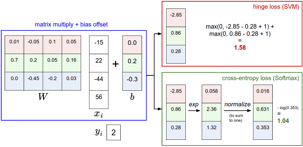
The label $y_i=2$ uses zero-based indexing: class $2$ is the third entry. Its logit is $0.28$, not the largest logit. Following the diagram’s rounded probabilities gives

We can check how softmax produced the probability needed for that last step. As in the previous lesson, subtract the largest logit, $0.86$, from all three scores without changing the probabilities:

Exponentiating gives approximately $(0.0245,1,0.5599)$. Divide the correct class’s value by the sum of all three:

Then $L=-\ln (0.3534)\approx 1.04$. Small differences in the final decimal come from rounding. Notice that taking the logarithm of the correct logit, $0.28$, would be a different and incorrect calculation: cross-entropy takes the logarithm of the correct probability.

What the number tells you

A few values establish the scale:

Loss provides more information than whether the top-ranked class is correct. Predictions assigning $0.90$ and $0.50$ to the true class receive different losses, even if both rank it first. Likewise, the model in the diagram ranks the second class first, but the loss is calculated using the third class because that is the known answer.

For this lesson, the complete procedure is: obtain the softmax probabilities, identify the true class, select its probability, and compute its negative natural logarithm. Do not substitute the target’s one-hot value of $1$ for the model’s predicted probability—the target tells you which entry to select, not what probability the model assigned.

Key takeaways

For one classification example, cross-entropy is $L=-\ln (p_{\text{correct}})$. The correct label selects an entry from the predicted probability distribution. High probability on that entry produces low loss; low probability produces high loss. The same calculation will later apply when a model assigns probabilities to possible next tokens in text.

Next, you’ll begin tracing how a change in one quantity affects another using the chain rule.