Applying the Chain Rule to Two-Operation Computation Graphs

Welcome back. Last time, you turned a model’s probability for the correct class into a cross-entropy loss. That gave you a way to measure an error. Today’s question is different: if an input changes slightly, how much does the final output change?

You’ll use the chain rule to answer that question for a computation with two operations. This is the small-scale version of the calculation that lets a neural network find gradients of its loss. Allow about 35–40 minutes for the video and the worked examples.

One computation, two operations

Consider a number $x$ that is first processed by a function $f$. Call the intermediate result $u$. A second function $g$ turns $u$ into the final result $y$:

A computation graph keeps these operations separate. The image below shows that structure; its $f(x)$ is the intermediate value we are calling $u$.

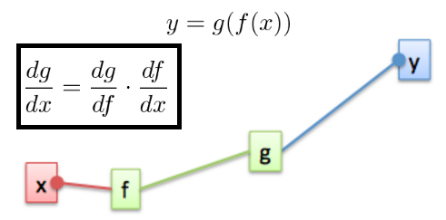
Suppose a small change in $x$ produces about three times that change in $u$. If a small change in $u$ then produces about twice that change in $y$, the change in $y$ is about six times the original change in $x$. The chain rule expresses this multiplication of local rates of change:

A derivative here is a rate of change at a particular input value. The important detail is that the outer function’s derivative, $g^{\prime }$, is evaluated at the intermediate value $u$, not necessarily at the original input $x$.

Forward values, backward gradients

Watch the two-operation example in Michigan Online’s Lecture 6: Backpropagation. The lecturer uses an addition operation followed by a multiplication operation. Pay attention to the difference between calculating the output and calculating how sensitive that output is to an input.

Here is that calculation in compact form. The graph has three inputs and two operations:

With $x=-2$, $y=5$, and $z=-4$, the forward pass calculates $q=3$ and then $F=-12$. Keeping $q=3$ available matters: its value is needed when calculating a gradient.

The backward pass starts at the final result. The derivative of $F$ with respect to itself is $1$. At the multiplication operation, changing $q$ while holding $z$ fixed changes $F$ at a rate of $z=-4$. Changing $z$ while holding $q$ fixed changes $F$ at a rate of $q=3$:

The addition operation has a local derivative of $1$ with respect to either of its inputs. To find the effect of $x$ on the final result, multiply the gradient already found at $q$ by that local derivative:

The same reasoning gives $\partial F/\partial y=-4$. These are partial derivatives: when considering a change to one input, the other inputs are held fixed. Notice that $z$’s gradient is $3$, while $x$’s and $y$’s are $-4$. Their routes through the graph differ, even though they all influence $F$.

Apply the rule to a single-input graph

Let’s use the structure in the image with two different operations:

At $x=1$, calculate the forward values first. The intermediate value is $u=3$, and the final value is $y=9$.

Now work backward. For the squaring operation, $dy/du=2u$, which equals $6$ at $u=3$. For the first operation, $du/dx=2$. Therefore,

The result says that near $x=1$, a small increase of $0.01$ in $x$ should increase $y$ by roughly $0.12$. As a check, at $x=1.01$, the exact output is $3.02^2=9.1204$, an increase of $0.1204$. The derivative gives the local approximation; it need not predict a finite change exactly.

This example also shows a common mistake. Substituting $x=1$ directly into $g^{\prime }(u)=2u$ would give $2$, not $6$. The squaring operation receives $u=3$, so its derivative must be evaluated there.

Connecting gradients to loss

The final output of a training computation is often a loss, like the cross-entropy loss from the previous lesson. For one correct-class probability $p$, you learned that $L=-\ln p$. Imagine a deliberately simplified two-operation model that sets $p=w/4$, with $0<w<4$. Its operations are:

At $w=2$, the forward pass gives $p=0.5$ and $L=-\ln (0.5)\approx 0.693$. The local derivative of the loss operation is $dL/dp=-1/p=-2$ at $p=0.5$. The local derivative of the probability operation is $dp/dw=1/4$. Chaining them gives

This linear rule for $p$ is a toy example, not how a real classifier normally computes probabilities. Its purpose is to make the chain rule visible: the negative gradient tells us that, near $w=2$, increasing $w$ slightly would decrease this example’s loss. Finding that gradient and deciding how to change $w$ are separate tasks; the latter is the subject of the next lesson.

Key takeaways

For a two-operation graph, calculate intermediate values in the forward pass. Then, working from the output backward, multiply the gradient from the later operation by the earlier operation’s local derivative. Evaluate each local derivative at the value that operation actually received.

That is the chain rule behind backpropagation. Next, you’ll take a supplied gradient and use it to perform one gradient-descent parameter update.