Perform a Gradient-Descent Parameter Update

Recommended resources

The freely available resources this lesson will direct you to.

Welcome back. In the previous lesson, you used the chain rule to find how a loss changes when a parameter changes. In the toy example, the loss gradient at $w = 2$ was $- 0.5$ . That gradient is information about the loss; it has not changed the parameter yet.

Today you’ll use a supplied gradient to make one gradient-descent update. You’ll see why the gradient’s sign determines the direction of the change, why the learning rate determines its size, and how the same rule applies when a model has several parameters. Allow about 35 minutes for the video, reading, and worked calculations.

From a gradient to a new parameter

Let $w$ be a parameter and $L$ the loss we want to reduce. If a supplied gradient $d L / d w$ is positive, increasing $w$ slightly would increase the loss locally, so a small decrease in $w$ is sensible. If the gradient is negative, a small increase in $w$ is sensible. Gradient descent moves opposite the gradient.

Watch DeepLearningAI’s Gradient Descent (C1W2L04) for a visual account of that sign rule. The clip uses a loss curve with one adjustable parameter; you do not need the earlier logistic-regression material to follow this portion.

Gradient Descent (C1W2L04)

DeepLearningAI’s Gradient Descent (C1W2L04) shows how a derivative becomes a parameter change and why subtracting it moves toward lower loss locally.

Watch the update rule for the roles of the parameter, gradient, and learning rate. Continue with the sign check: notice what subtraction does when the slope is positive versus negative.

For one parameter, the rule is

w_{new} = w_{old} - η \frac{d L}{d w}_{w_{old}},

where $η > 0$ is the learning rate. The vertical bar means that the supplied gradient was evaluated at the old parameter value. First multiply the gradient by the learning rate; then subtract that signed result from the old parameter.

The gradient answers which direction, and how steeply? The learning rate answers how large a change should we attempt? A negative gradient does not mean that we subtract a positive number: subtracting a negative quantity increases $w$ .

One complete update

Return to the previous lesson’s toy model. At $w_{old} = 2$ , you found the supplied gradient $d L / d w = - 0.5$ . Choose a learning rate of $η = 0.2$ . The update is

w_{new} = 2 - (0.2) (- 0.5) = 2.1.

The learning rate scales the gradient to $- 0.1$ ; subtracting that result increases the parameter by $0.1$ . This is one update, not a search for the final best value of $w$ .

In that toy model, $p = w /4$ and $L = - ln p$ . At $w = 2$ , the loss is approximately $0.693$ ; at $w = 2.1$ , it is approximately $0.644$ . The loss did decrease in this example. We can check because we know its formula, but calculating the new loss is not part of the arithmetic needed to perform the update from a supplied gradient.

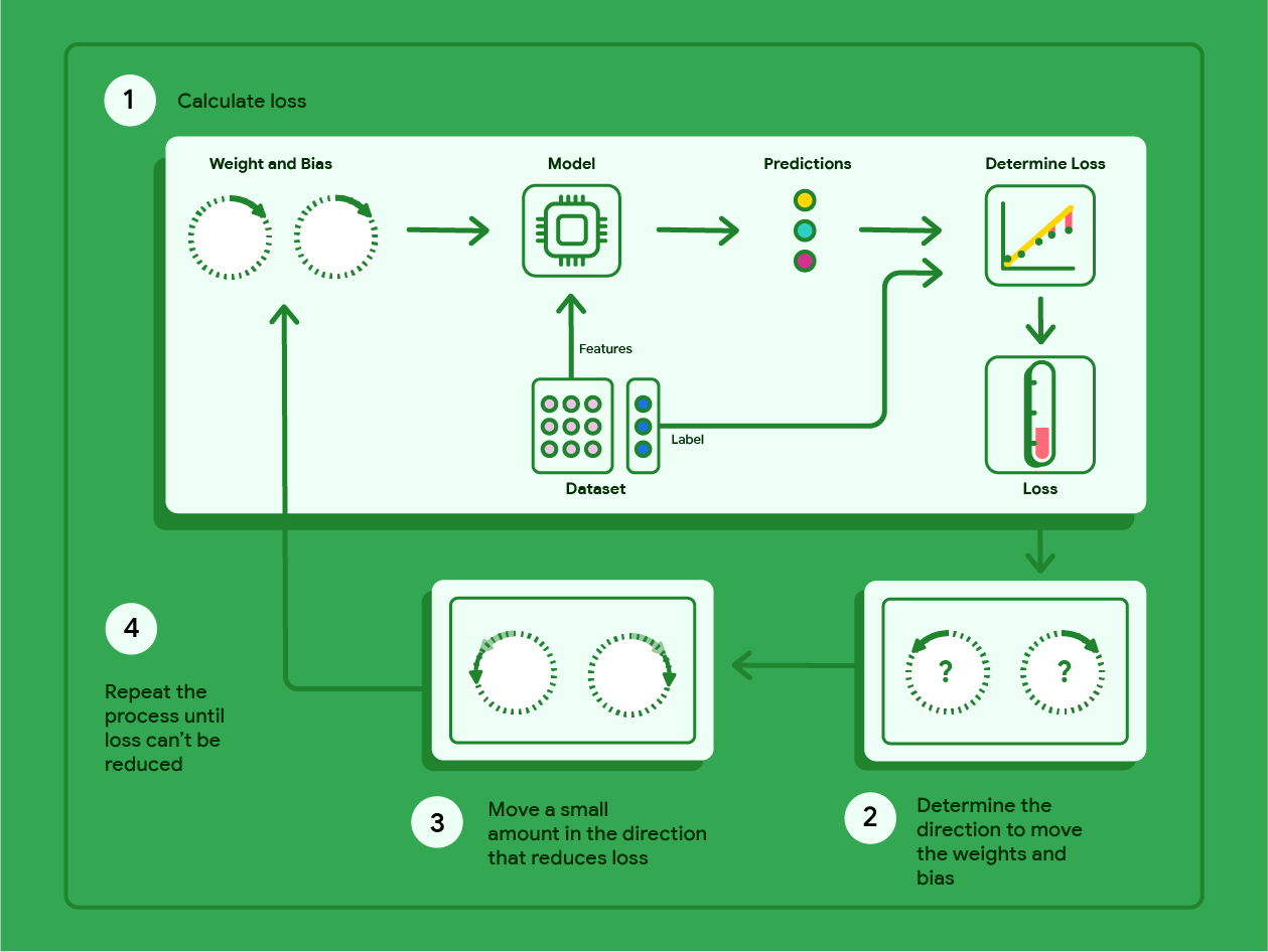
The distinction between one update and training matters. A training process calculates loss and gradients at its current parameter values, makes an update, and repeats. It cannot generally reuse the old gradient indefinitely: after $w$ changes, the slope of the loss may change too.

The numbered illustration shows a training cycle: calculate loss from predictions, determine how the parameters should change, make a small update, and repeat using the updated weights and bias. This lesson focuses on the parameter-change step.

Updating several parameters at once

A model usually has more than one adjustable number. Suppose its current parameters are a weight vector and a bias:

w_{old} = [0.4 - 1.0], b_{old} = 0.2.

Suppose the gradients supplied at those current values are

\nabla_{w} L = [0.5 - 0.3], \frac{\partial L}{\partial b} = - 0.4.

With $η = 0.1$ , apply the same rule to every component:

w_{new} = [0.4 - 1.0] - 0.1 [0.5 - 0.3] = [0.35 - 0.97],

b_{new} = 0.2 - (0.1) (- 0.4) = 0.24.

The first weight falls because its gradient is positive. The second weight and the bias rise because their gradients are negative. All three new values use gradients evaluated at the same old parameter values. You would need newly evaluated gradients before making another update.

In compact form, if $θ$ collects all the model’s parameters, the rule is

θ_{new} = θ_{old} - η \nabla_{θ} L .

The gradient has one entry per parameter, so the subtraction is componentwise. This is the bridge from the single-number calculation to the many weights of a neural network.

Why the learning rate matters

The gradient describes the loss near the current parameters. It does not guarantee that an arbitrarily large move opposite the gradient will lower the loss. Read the “Learning rate” subsection of Google’s Linear regression: Hyperparameters for the relationship between gradient size and update size.

Linear regression: Hyperparameters | Machine Learning

Read Google’s “Learning rate” subsection to connect the update arithmetic to the choice of step size.

In the subsection titled “Learning rate,” begin at the explanation of what happens when the rate changes and read through the final numerical example, which ends with a parameter change of 0.025. Focus on the difference between the magnitude of a change and its direction: the gradient’s sign is still needed to determine the latter.

A small numerical example makes the risk of a large step precise. Let $L (w) = (w - 1)^{2}$ , and start at $w = 3$ . The loss is $4$ , and the gradient there is $4$ . Different learning rates give different single updates from that same starting point:

Learning rate	Updated $w$	New loss
$0.01$	$3 - 0.01 (4) = 2.96$	$3.8416$
$0.1$	$3 - 0.1 (4) = 2.6$	$2.56$
$1.1$	$3 - 1.1 (4) = - 1.4$	$5.76$

All three updates move opposite the gradient at $w = 3$ . The largest step passes the minimum at $w = 1$ and lands at a higher loss than where it began. This is why “opposite the gradient” describes a locally promising direction, not a promise that every step size works.

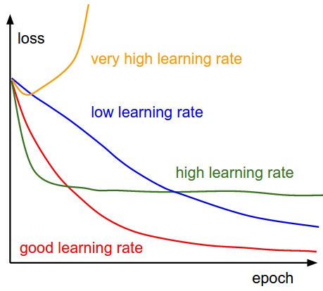
Schematic loss-versus-epoch curves: a very high learning rate rises sharply, a low rate decreases slowly, a high rate levels off, and a well-chosen rate decreases substantially. The curves illustrate possible training behavior, not a universal ranking of fixed learning-rate values.

An epoch is one pass through a training dataset. Unlike the table, which compares just one update, the image sketches what may happen across repeated updates. The useful question when reading such a plot is not merely “Did the loss go down on the first step?” but “Does the chosen rate allow useful progress over training?”

Key takeaways

To update a parameter from a supplied gradient, multiply the gradient by the positive learning rate and subtract the signed result from the old parameter. A positive gradient decreases that parameter; a negative gradient increases it. With several parameters, apply the rule componentwise using gradients evaluated at the same old parameter values. The learning rate controls step size, and too large a step can increase loss despite moving in the correct local direction.

You now have the core sequence: calculate a loss, find its gradients, and use them to change parameters. Next, you’ll turn to normalizing a feature vector using its mean and variance.