Feature Vector Normalization Using Mean and Variance

Welcome back. In the previous lesson, you used a gradient and a learning rate to update a model parameter. Before a model can learn effectively from numerical inputs, it often helps to put those inputs on a comparable scale.

This lesson focuses on one operation: subtract a feature vector’s mean, then divide by its standard deviation, which is calculated from its variance. You’ll work through the arithmetic by hand, then distinguish which values should be used to calculate the mean in a tabular dataset. Allow about 35 minutes.

---

Why change a feature’s scale?

Imagine a dataset with two input features: the number of rooms in a home and its floor area in square metres. Room counts might be single-digit numbers, while floor areas might be in the hundreds. Those numerical scales reflect different units, not necessarily different importance to the prediction.

For models trained with gradient descent, poorly matched feature scales can make optimization less straightforward. Watch the two short passages below for the basic operation and its connection to the updates you studied last time.

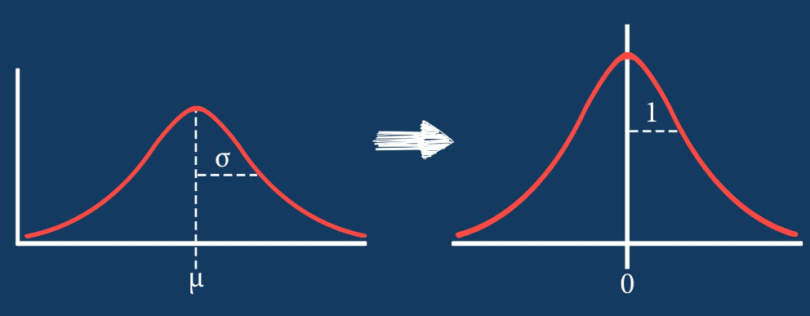
This operation is commonly called standardization or Z-score scaling. “Normalization” can mean several kinds of rescaling in machine learning; here, it means this particular mean-and-variance-based operation. It is useful to know the distinction because standardization does not squeeze every value into the interval from 0 to 1.

---

Mean, variance, and the Z-score

Read Google’s Numerical data: Normalization for the interpretation of a Z-score as a distance from the mean measured in standard deviations. The figures help connect the arithmetic to what happens to an entire feature’s values.

Suppose our feature vector contains $n$ values, $\mathbf{x}=(x_1,\dots ,x_n)$. First find its mean, the average value:

$$\mu =\frac{1}{n}\sum _{i=1}^n{x}_i.$$

Then find its variance, the average squared distance from that mean:

$$v=\frac{1}{n}\sum _{i=1}^n(x_i-\mu {)}^2.$$

The standard deviation is $\sigma =\sqrt{v}$. It brings the measure of spread back into the same units as the original values. When $\sigma >0$, standardize each entry with

$$z_i=\frac{x_i-\mu }{\sigma }=\frac{x_i-\mu }{\sqrt{v}}.$$

Subtracting $\mu$ centres the values at zero. Dividing by $\sigma$ expresses each centred value in units of standard deviation. Notice that we divide by the square root of variance, not by variance itself.

For this complete vector, we use $n$ in the variance calculation. You may encounter a formula that divides by $n-1$ when estimating variance from a sample; that is a different statistical purpose. Use the convention specified for the normalization you are performing.

---

Normalize a vector by hand

Take the vector

$$\mathbf{x}=(2,4,6,8).$$

Its mean is

$$\mu =\frac{2+4+6+8}{4}=5.$$

Subtract 5 from every entry to obtain the centred vector $(-3,-1,1,3)$. Square those deviations and average them:

$$v=\frac{(-3{)}^2+(-1{)}^2+1^2+3^2}{4}=\frac{20}{4}=5.$$

The standard deviation is therefore $\sqrt{5}$, giving the normalized vector

$$\mathbf{z}=\left(-\frac{3}{\sqrt{5}},-\frac{1}{\sqrt{5}},\frac{1}{\sqrt{5}},\frac{3}{\sqrt{5}}\right)\approx (-1.342,-0.447,0.447,1.342).$$

The first entry is about 1.342 standard deviations below the original mean; the last is about 1.342 standard deviations above it. The vector still has four entries. We have changed their values, not the vector’s shape.

There is a useful way to check the result. The entries sum to zero, so their mean is zero. Their squared values sum to $20/5=4$; averaging over four entries gives variance 1. Those are the two defining properties of standardization when the original variance is nonzero.

---

Which values supply the mean and variance?

The arithmetic above works for any chosen group of values, but choosing the group correctly matters. In a tabular dataset, a feature is usually a column: for example, floor area measured across many homes. You calculate one mean and one variance for that column, then use them to transform each value in it. You calculate a separate pair of statistics for a different feature such as room count. Averaging floor area and room count together within one home would mix different units and would not standardize either feature across the dataset.

For example, if the room-count column were $(2,4,6,8)$, its fitted mean and variance would be 5 and 5, as calculated above. A new home with 7 rooms would be transformed using those same statistics:

$$z_{\text{new}}=\frac{7-5}{\sqrt{5}}\approx \mathrm{0.894.}$$

You would not recalculate the mean from the new home’s features. In a training workflow, fit the statistics on the training data and reuse them for validation, test, and later inputs; otherwise, information from held-out data can leak into preprocessing.

There is one important boundary case. If every value in a feature vector is identical, its variance and standard deviation are zero, so the formula would divide by zero. Implementations need an explicit rule for this case. In neural-network calculations, one common form adds a small positive constant $\epsilon$ inside the square root:

$$z_i=\frac{x_i-\mu }{\sqrt{v+\epsilon }}.$$

This makes the calculation defined when $v=0$, although a constant vector then remains all zeros and cannot have variance 1. For nonconstant vectors, adding $\epsilon$ also makes the resulting variance slightly different from 1.

Later, when you study Transformer layer normalization, you’ll meet the same centre-and-scale arithmetic with a different choice of values: the features within a token representation. For now, keep the general rule in view: identify the group being normalized, compute its mean and variance, and use those statistics consistently.

---

Key takeaways

To normalize a feature vector using mean and variance, calculate the mean, average the squared deviations to get variance, and divide each centred entry by the standard deviation. For a nonconstant vector, the result has mean 0 and variance 1. Standardization changes centre and scale; it does not guarantee values between 0 and 1 or make a skewed distribution bell-shaped.

You have now completed the mathematical groundwork in this module. Next, you’ll create PyTorch tensors and identify their batch, sequence, and feature dimensions—skills you will use to track how data moves through a neural network.