SVD from Eigendecomposition of AᵀA

Introduction

In our previous lesson, we developed a powerful geometric intuition for the Singular Value Decomposition (SVD). We saw that any linear transformation represented by a matrix $A$ can be universally decomposed into a sequence of three fundamental operations: a rotation ($V^T$), a scaling ($\Sigma$), and a final rotation ($U$). This gives us the elegant equation $A=U\Sigma V^T$.

While this geometric picture is fundamental, it doesn't yet tell us how to find the matrices $U$, $\Sigma$, and $V$ for a given matrix $A$. Today, we will bridge that gap. We will derive the complete algebraic procedure for computing the SVD, starting from first principles. The key to this derivation is a clever trick: we will construct a special symmetric matrix from $A$, allowing us to leverage the power of eigendecomposition, which we've already studied.

The Key: Constructing a Symmetric Matrix

As we know, eigendecomposition is most powerful when applied to symmetric matrices, which are guaranteed to have real eigenvalues and a full set of orthogonal eigenvectors (the Spectral Theorem). Our matrix $A$, however, may be non-symmetric or even rectangular.

This brings us to a crucial question. Given a general $m\times n$ matrix $A$, how can you combine it with its transpose, $A^T$, to construct a new matrix that is guaranteed to be both square and symmetric?

Answer

There are two ways: you can compute $A^TA$ (which will be an $n \times n$ matrix) or $AA^T$ (which will be an $m \times m$ matrix). Both are square and symmetric. You can verify this for $A^TA$ by taking its transpose: $(A^TA)^T = A^T(A^T)^T = A^TA$.

This simple construction is the key that unlocks the SVD. Let's focus on the matrix $S=A^{T}A$. This matrix is not just symmetric; it also has another special property: it is positive semi-definite. This means all of its eigenvalues are non-negative ($\lambda \ge 0$). This is a critical property, as we will soon need to take the square root of these eigenvalues.

To see why this is true, let's watch a short, rigorous proof.

Deriving the Connection to Eigendecomposition

Now that we have a symmetric, positive semi-definite matrix $S=A^{T}A$, we can explore its relationship to the SVD formula, $A=U\Sigma V^T$. Let's substitute this formula into the expression for $S$:

$$S=A^{T}A=(U\Sigma V^T{)}^T(U\Sigma V^T)$$

Using the property that $(XYZ{)}^T=Z^T{Y}^T{X}^T$, we get:

$$A^{T}A=(V{\Sigma }^T{U}^T)(U\Sigma V^T)$$

Since the left singular vectors in $U$ form an orthonormal basis, the matrix $U$ is orthogonal, which means $U^{T}U=I$. The expression simplifies beautifully:

$$A^{T}A=V({\Sigma }^T\Sigma )V^T$$

Now, take a close look at this final equation. It has the form Matrix = P * D * P⁻¹ (or P * D * Pᵀ since V is orthogonal).

Question: What does this equation represent? What does it tell us about the matrices $V$ and $({\Sigma }^T\Sigma )$ in relation to the matrix $A^{T}A$?

Answer

This is precisely the **eigendecomposition of the symmetric matrix $A^TA$**.

This implies two profound connections:

1. The columns of the matrix $V$ are the orthonormal eigenvectors of $A^{T}A$.
2. The matrix $({\Sigma }^T\Sigma )$ is a diagonal matrix containing the eigenvalues of $A^{T}A$.

From this, we can deduce the recipe for finding the components of the SVD. The matrix $\Sigma$ is an $m\times n$ matrix that is zero everywhere except for its main diagonal. The product ${\Sigma }^T\Sigma$ is an $n\times n$ diagonal matrix whose diagonal entries are ${\sigma }_i^2$.

Therefore, the eigenvalues of $A^{T}A$ are the squares of the singular values of $A$.

$${\lambda }_i(A^{T}A)={\sigma }_i^2(A)$$

This means the singular values of $A$ are the square roots of the eigenvalues of $A^{T}A$: ${\sigma }_i=\sqrt{{\lambda }_i}$. This is why the positive semi-definite property we proved earlier is so important!

The Algorithm for Computing SVD

We have now established all the necessary connections to outline a concrete algorithm for finding the SVD of any matrix $A$. The following resource provides a crisp summary of the steps.

Let's consolidate that information.

Step 1: Find $V$ and $\Sigma$.

1. Construct the symmetric matrix $S=A^{T}A$.
2. Compute the eigendecomposition of $S$ to find its eigenvalues ${\lambda }_1,{\lambda }_2,\dots ,{\lambda }_n$ and corresponding orthonormal eigenvectors ${\vec{v}}_1,{\vec{v}}_2,\dots ,{\vec{v}}_n$.
3. The right singular vectors are the eigenvectors of $A^{T}A$. Construct the matrix $V$ by placing these eigenvectors as its columns: $V=[{\vec{v}}_1|{\vec{v}}_2|\dots |{\vec{v}}_n]$.
4. The singular values are the square roots of the eigenvalues: ${\sigma }_i=\sqrt{{\lambda }_i}$. By convention, we sort these in descending order, ${\sigma }_1\ge {\sigma }_2\ge \cdots \ge 0$.
5. Construct the $m\times n$ matrix $\Sigma$ by placing these singular values on its main diagonal.

Step 2: Find $U$.

1. Recall the fundamental relationship from our last lesson: $A{\vec{v}}_i={\sigma }_i{\vec{u}}_i$.
2. For all non-zero singular values (${\sigma }_i>0$), we can find the corresponding left singular vectors ${\vec{u}}_i$ by rearranging this equation: $${\vec{u}}_i=\frac{1}{{\sigma }_i}A{\vec{v}}_i$$
3. These vectors form the first $r$ columns of $U$, where $r$ is the rank of the matrix $A$.
4. If $A$ is not full rank or is rectangular ($m>r$), we will have found fewer than $m$ columns for $U$. The remaining $m-r$ columns must be vectors that are orthonormal to the ones we've already found. These vectors form an orthonormal basis for the null space of $A{A}^T$, also known as the left null space of $A$. We can find them using a method like the Gram-Schmidt process.

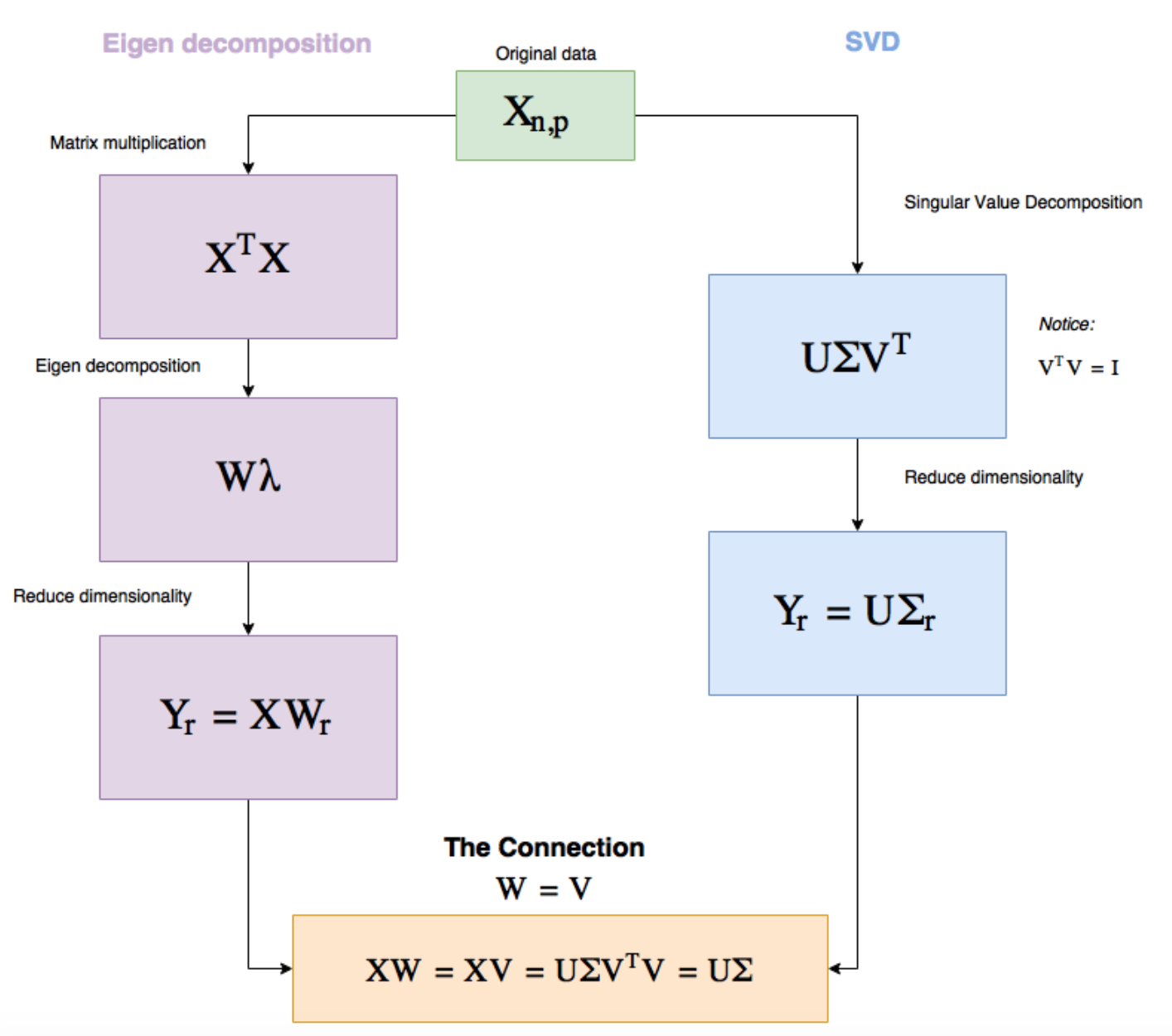
The following flowchart provides a great visual summary of how the SVD calculation relates to the eigendecomposition of $A^{T}A$.

A Worked Example

Let's solidify this procedure by walking through a complete example. Decomposing a non-square matrix is particularly illustrative, as it forces us to handle the dimensions of $\Sigma$ carefully and to consider the case where we must complete the basis for $U$.

The example highlights that the derivation $A^{T}A=V({\Sigma }^T\Sigma )V^T$ is not just a theoretical curiosity; it is the blueprint for a practical algorithm to compute the Singular Value Decomposition of any matrix.

Conclusion

In this lesson, we transitioned from the geometric what of SVD to the algebraic how. We established a rigorous procedure to compute the $U$, $\Sigma$, and $V$ matrices for any given matrix $A$.

Key Takeaways:

• Symmetric Matrix Construction: The key to deriving SVD is to form the symmetric, positive semi-definite matrix $A^{T}A$.
• Connection to Eigendecomposition: The eigendecomposition of $A^{T}A$ directly reveals two of the SVD components. The equation $A^{T}A=V({\Sigma }^T\Sigma )V^T$ shows that:
  • The columns of $V$ are the eigenvectors of $A^{T}A$.
  • The singular values in $\Sigma$ are the square roots of the eigenvalues of $A^{T}A$.
• Completing the Decomposition: The left singular vectors in $U$ are found using the fundamental relationship $A{\vec{v}}_i={\sigma }_i{\vec{u}}_i$. If necessary, the basis for $U$ is completed by finding an orthonormal basis for the left null space of $A$.

We now have both a deep geometric intuition and a concrete computational algorithm for SVD. With this foundation, we are ready to explore its applications. In the next lesson, we will examine one of the most important uses of SVD: low-rank approximation. This powerful technique allows us to find the best possible simplified version of a matrix, forming the mathematical core of methods like Principal Component Analysis (PCA), data compression, and modern techniques for learning compressed representations in neural networks.