Low-Rank Approximation with SVD

Introduction

In our last lesson, we developed a complete algebraic algorithm for computing the Singular Value Decomposition (SVD), $A=U\Sigma V^T$, by leveraging the eigendecomposition of the symmetric matrix $A^{T}A$. We now understand not only the geometric meaning of SVD as a sequence of rotation-scaling-rotation but also the precise method for finding the matrices $U$, $\Sigma$, and $V$.

Today, we delve into one of the most consequential applications of SVD: low-rank approximation. The central idea is to find a "simpler" matrix of a lower rank that is as close as possible to our original matrix. This technique is the mathematical engine behind a vast array of methods, from data compression and dimensionality reduction to optimizing performance-critical operations in computer graphics. For you, this concept forms the bridge between classical linear algebra and the modern idea of learning compressed or "latent" representations in neural networks like autoencoders.

SVD as a Sum of Rank-One Matrices

To understand how SVD enables approximation, we first need to look at its structure from a different perspective. Instead of viewing $A=U\Sigma V^T$ as a product of three matrices, we can expand it into a sum.

Let's write out the matrices: $U$ has columns ${\vec{u}}_i$, $V$ has columns ${\vec{v}}_i$ (so $V^T$ has rows ${\vec{v}}_i^T$), and $\Sigma$ has diagonal entries ${\sigma }_i$. The product can be expressed as:

$$A=\sum _{i=1}^r{\sigma }_i{\vec{u}}_i{\vec{v}}_i^T$$

where $r$ is the rank of matrix $A$. Each term in this sum, ${\vec{u}}_i{\vec{v}}_i^T$, is an outer product of two vectors. An $m\times 1$ column vector ${\vec{u}}_i$ multiplied by a $1\times n$ row vector ${\vec{v}}_i^T$ results in an $m\times n$ matrix.

Question: What is the rank of a matrix formed by the outer product of two non-zero vectors, like ${\vec{u}}_i{\vec{v}}_i^T$? Why?

Answer

The rank is exactly **one**. Every column of the resulting matrix is just the vector $\vec{u}_i$ scaled by a different element of $\vec{v}_i^T$. Therefore, all columns are linearly dependent on a single vector, $\vec{u}_i$, meaning the column space has a dimension of one.

This means the SVD elegantly decomposes any matrix $A$ into a weighted sum of rank-one matrices. The singular values ${\sigma }_i$, which are sorted in descending order (${\sigma }_1\ge {\sigma }_2\ge \cdots \ge {\sigma }_r>0$), act as the weights. This tells us that the first term, ${\sigma }_1{\vec{u}}_1{\vec{v}}_1^T$, is the most significant rank-one component of the matrix. The second term is the next most significant, and so on.

Let's watch a clear explanation of this expansion.

Truncated SVD and the "Best" Approximation

Now that we see $A$ as a sum of weighted components, the idea of approximation becomes natural. If the singular values ${\sigma }_i$ drop off in magnitude quickly, perhaps we can get a very good approximation of $A$ by keeping only the first few, most significant terms and discarding the rest.

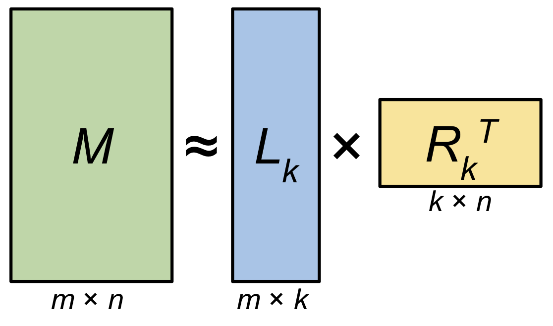
This is the core idea of low-rank approximation. We can create an approximation of $A$, let's call it ${\tilde{A}}_k$, by truncating the sum after $k$ terms, where $k<r$:

$${\tilde{A}}_k=\sum _{i=1}^k{\sigma }_i{\vec{u}}_i{\vec{v}}_i^T$$

This is equivalent to forming the matrix product using only the first $k$ singular values and their corresponding singular vectors:

$${\tilde{A}}_k=U_k{\Sigma }_k{V}_k^T$$

where $U_k$ contains the first $k$ columns of $U$, ${\Sigma }_k$ is the top-left $k\times k$ block of $\Sigma$, and $V_k$ contains the first $k$ columns of $V$. Since ${\tilde{A}}_k$ is a sum of $k$ rank-one matrices, its rank is at most $k$.

This is an approximation, but is it a good one? In fact, it is the best possible approximation of rank $k$. This remarkable result is formalized by the Eckart-Young-Mirsky Theorem.

The theorem addresses the following optimization problem: find the matrix $B$ of rank $k$ that is "closest" to $A$. We measure "closeness" using the Frobenius norm, which is the matrix equivalent of the Euclidean vector norm:

$$\Vert A-B{\Vert }_F=\sqrt{\sum _{i=1}^m\sum _{j=1}^n(A_{ij}-B_{ij}{)}^2}$$

The theorem states that the rank-$k$ matrix $B$ that minimizes this error is precisely the truncated SVD, ${\tilde{A}}_k$.

To formalize this, let's turn to a set of lecture notes that states the theorem and provides the proof from first principles.

The Eckart-Young theorem is profound. It guarantees that we don't need to search through the infinite space of all possible rank-$k$ matrices. The optimal solution is handed to us directly by the SVD.

Application 1: Image Compression

A classic and highly intuitive application of low-rank approximation is image compression. A grayscale image can be represented as a matrix where each entry is a pixel's intensity. A color image can be three such matrices (for Red, Green, and Blue channels).

By taking the SVD of an image matrix and keeping only the top $k$ singular components, we can reconstruct an approximation of the image. The compression comes from the storage requirements. To store the full $m\times n$ image, we need $mn$ numbers. To store the rank-$k$ approximation, we need to store $U_k$ ($m\times k$), ${\Sigma }_k$ ($k$ values), and $V_k$ ($n\times k$), for a total of $mk+k+nk=k(m+n+1)$ values. If $k$ is small, this is a substantial saving.

Let's see this in action.

Application 2: Approximating Filters in Computer Graphics

This application connects directly to your interests in graphics and high-performance systems. In image processing, we often apply 2D filters (kernels) to an image to achieve effects like blurring, sharpening, or edge detection. This is done via a 2D convolution.

A $K\times K$ filter is called separable if it can be written as the outer product of two 1D vectors (a column and a row). Applying a separable filter is much faster than a non-separable one. Instead of $K^2$ operations per pixel, we can perform two passes with $K$ operations each, reducing the complexity from $O(K^2)$ to $O(K)$.

This is a linear algebra problem in disguise: a filter matrix is separable if and only if it has a rank of one.

What can we do for non-separable filters, like a circular or hexagonal kernel used for simulating camera bokeh? We can use SVD to find the best rank-1 approximation, which gives us the closest possible separable filter.

If the rank-1 approximation isn't good enough, we can use a rank-$k$ approximation. This corresponds to summing $k$ independent separable filters. This is still vastly more efficient than a full 2D convolution if $k$ is small.

The following blog post from a graphics engineer provides an excellent, practical overview.

Conclusion

In this lesson, we have unlocked a truly powerful application of the SVD. By re-interpreting the decomposition as a weighted sum of rank-one matrices, we developed the idea of low-rank approximation by truncating this sum.

Key Takeaways:

• SVD as a Sum: Any matrix $A$ can be decomposed into $A={\sum }_{i=1}^r{\sigma }_i{\vec{u}}_i{\vec{v}}_i^T$, a sum of rank-one matrices weighted by their singular values.
• Optimal Approximation: The Eckart-Young-Mirsky theorem guarantees that the best rank-$k$ approximation of a matrix $A$ (in the Frobenius norm sense) is given by the truncated SVD, ${\tilde{A}}_k=U_k{\Sigma }_k{V}_k^T$.
• Concentration of Energy: The rapid decay of singular values for many real-world matrices (like images) means that a low-rank approximation can capture most of the original information with significantly less data.
• Practical Applications: This principle is the foundation for data compression (images, signals) and performance optimization in domains like computer graphics (filter approximation).

We are now nearing the end of our foundational module on linear algebra. In the next lesson, we will cover our final topic in this area: orthogonal projection. This concept is not only geometrically elegant but also provides the direct solution to the fundamental problem of Ordinary Least Squares, which will be our entry point into the world of optimization. Following that, we will briefly touch on Principal Component Analysis (PCA) as a self-study topic, as it is a direct application of the eigendecomposition and low-rank approximation concepts we've mastered.