Orthogonal Projections onto Subspaces

Recommended resources

The freely available resources this lesson will direct you to.

Introduction

In our last lesson, we saw how the Singular Value Decomposition (SVD) provides the optimal low-rank approximation of a matrix, a principle with powerful applications in compression and performance optimization. Today, we explore a different, yet related, kind of "best approximation": finding the closest vector in a subspace to a vector outside of it. This is the problem of orthogonal projection.

This concept is not just a cornerstone of geometric linear algebra; it forms the very foundation of linear regression and optimization. Understanding projection is the crucial first principles step to understanding Ordinary Least Squares (OLS), which is the classical ancestor of the optimization algorithms used in deep learning. Our goal is to derive, from scratch, the formula for projecting a vector onto any subspace and to understand its deep geometric significance.

The Simplest Case: Projection onto a Line

Let's begin with the most intuitive case: projecting a vector onto a line. Imagine a vector $b$ in $R^{n}$ and a line passing through the origin, which is spanned by another vector $a$ . We want to find the vector $p$ on that line that is closest to $b$ .

An illustration of projecting a 3D object onto a 2D plane. We will start with an even simpler case: projecting a vector onto a 1D line.

The vector $p$ is the "shadow" that $b$ casts onto the line defined by $a$ . The key insight comes from the error vector, $e = b - p$ , which connects the projection $p$ to the original vector $b$ . For $p$ to be the closest point, this error vector must be orthogonal (perpendicular) to the line itself, and therefore orthogonal to the vector $a$ that spans it.

This single geometric condition, $a ⊥ (b - p)$ , is all we need.

The Projection $p$ in terms of $a$ : Since $p$ lies on the line spanned by $a$ , it must be a scalar multiple of $a$ . We can write $p = x^a$ , where $x^$ is some scalar we need to find.
The Orthogonality Condition: The dot product of two orthogonal vectors is zero. So, our condition becomes:
$a^{T} (b - p) = 0$

Now, let's use these two facts to solve for $x^$ .

Question: Substitute the expression for $p$ into the orthogonality condition and solve for the scalar $x^$ . What do you get?

Answer

Substituting $\vec{p} = \hat{x}\vec{a}$ into the equation gives: $$ \vec{a}^T (\vec{b} - \hat{x}\vec{a}) = 0 $$ Distributing the transpose: $$ \vec{a}^T\vec{b} - \hat{x}\vec{a}^T\vec{a} = 0 $$ Since $\vec{a}^T\vec{a}$ is just a scalar (the squared length of $\vec{a}$), we can solve for $\hat{x}$: $$ \hat{x} = \frac{\vec{a}^T\vec{b}}{\vec{a}^T\vec{a}} $$

With this, we have everything. The projection vector $p$ is:

p = x^a = (\frac{a ^{T} b}{a ^{T} a}) a

Notice the numerator is the dot product of $a$ and $b$ , and the denominator is the squared L2 norm of $a$ .

Professor Gilbert Strang's lecture on this topic is a classic for a reason. Let's watch his derivation to solidify this fundamental idea.

15. Projections onto Subspaces

In his MIT OpenCourseWare lecture "Projections onto Subspaces," Professor Strang masterfully explains the geometry and derives the formulas for projection.

Watch the first part of the lecture, from the beginning to the end of the 1D case. He will cover the geometry, the derivation of \hat{x}, the projection vector \vec{p}, and introduce the idea of a projection matrix.

As Professor Strang highlights, we can also express this operation with a projection matrix, $P$ . The projection $p$ is a linear transformation of $b$ , so we're looking for a matrix $P$ such that $p = P b$ . By rearranging our formula for $p$ (remembering that scalars can be moved around), we get:

p = a (\frac{a ^{T} b}{a ^{T} a}) = \frac{a a ^{T}}{a ^{T} a} b

This gives us the projection matrix for projecting onto the line spanned by $a$ :

P = \frac{a a ^{T}}{a ^{T} a}

Note the structure: the denominator $a^{T} a$ is an inner product (a scalar), while the numerator $a a^{T}$ is an outer product (a rank-one matrix), a concept we encountered in the last lesson.

Projection onto a General Subspace

Now, let's generalize. Instead of a line (a 1D subspace), what if we want to project a vector $b$ onto a $k$ -dimensional subspace $W$ ?

This is the central problem of least squares. Often, a system of linear equations $A x = b$ has no solution. This happens when $b$ is not in the column space of $A$ . Since we can't find an $x$ that produces $b$ exactly, we settle for the next best thing: we find the vector $p$ in the column space of $A$ that is closest to $b$ . We then solve $A x^= p$ instead. This vector $p$ is the orthogonal projection of $b$ onto the column space of $A$ .

Let's formalize this. Let the subspace $W$ be the column space of a matrix $A$ , whose columns $a_{1}, \dots, a_{k}$ are linearly independent and form a basis for $W$ .

The Projection $p$ in terms of $A$ : Since $p$ is in the column space of $A$ , it must be a linear combination of its columns. We can write $p = A x^$ for some vector of coefficients $x^= [x^_{1}, \dots, x^_{k}]^{T}$ . Our goal is to find this vector $x^$ .
The Orthogonality Condition: The error vector, $e = b - p$ , must be orthogonal to the entire subspace $W$ . This means it must be orthogonal to every basis vector of $W$ .
$a_{1}^{T} (b - A x^) = 0 a_{2}^{T} (b - A x^) = 0 ⋮ a_{k}^{T} (b - A x^) = 0$

This system of $k$ equations can be written beautifully as a single matrix equation:

A^{T} (b - A x^) = 0

This equation is profound. It states that the error vector $b - A x^$ lies in the nullspace of $A^{T}$ . From our study of the four fundamental subspaces, we know that the nullspace of $A^{T}$ is the orthogonal complement of the column space of $A$ . This is a perfect confirmation of our geometric intuition!

Now, let's solve for $x^$ . Rearranging the equation, we get:

A^{T} A x^= A^{T} b

This is the famous Normal Equation. It's a symmetric system of $k \times k$ linear equations for the unknown coefficients $x^$ .

Assuming the matrix $A^{T} A$ is invertible (which it is, if the columns of $A$ are linearly independent), we can solve for $x^$ :

x^= (A^{T} A)^{- 1} A^{T} b

This gives us the coefficients for the best approximation. To get the projected vector $p$ itself, we multiply by $A$ :

p = A x^= A (A^{T} A)^{- 1} A^{T} b

And just like before, this gives us the general projection matrix for projecting onto the column space of $A$ :

P = A (A^{T} A)^{- 1} A^{T}

Let's return to Professor Strang's lecture, where he derives this exact result.

15. Projections onto Subspaces

We'll now see the generalization of our 1D case to any subspace.

First, watch the segment on why we project. This motivates the problem by framing it as finding the "best" solution to an unsolvable system A\vec{x}=\vec{b}. Next, watch from projecting onto a plane. This section builds the geometric argument and arrives at the crucial normal equation: A^T(\vec{b} - A\vec{\hat{x}}) = \vec{0}. Finally, see the solution from deriving the final formulas. Here, he solves the normal equation to find \vec{\hat{x}}, \vec{p}, and the general projection matrix P. Pay attention to his discussion of the properties P^T = P and P^2 = P, which are characteristic of all projection matrices.

To reinforce these steps with a clear, written derivation and a worked example, let's consult a supplementary text.

Orthogonal Projections

This document by Dan Klain provides a concise and formal derivation of the projection matrix.

Read the first two pages, from the start down to the end of the derivation of the projection matrix Q. This provides a compact summary of the logic we just developed. On page 3, read the short proof for why the matrix A^TA is invertible. This is a crucial assumption we made, and it's good to see it justified. Finally, work through the example on page 3 and its solution. Following the concrete numbers will help solidify the abstract formula.

A Very Important Special Case: Orthonormal Basis

The general formula $P = A (A^{T} A)^{- 1} A^{T}$ can be computationally intensive due to the matrix inverse. However, if our basis vectors for the subspace $W$ are orthonormal, the formula simplifies dramatically.

Let the matrix $Q$ have orthonormal columns (so $q_{i}^{T} q_{j} = 0$ for $i \neq = j$ and $q_{i}^{T} q_{i} = 1$ ). What does the term $Q^{T} Q$ become? It becomes the identity matrix, $I$ .

Question: Given that $Q^{T} Q = I$ , what does the general projection matrix formula $P = Q (Q^{T} Q)^{- 1} Q^{T}$ simplify to?

Answer

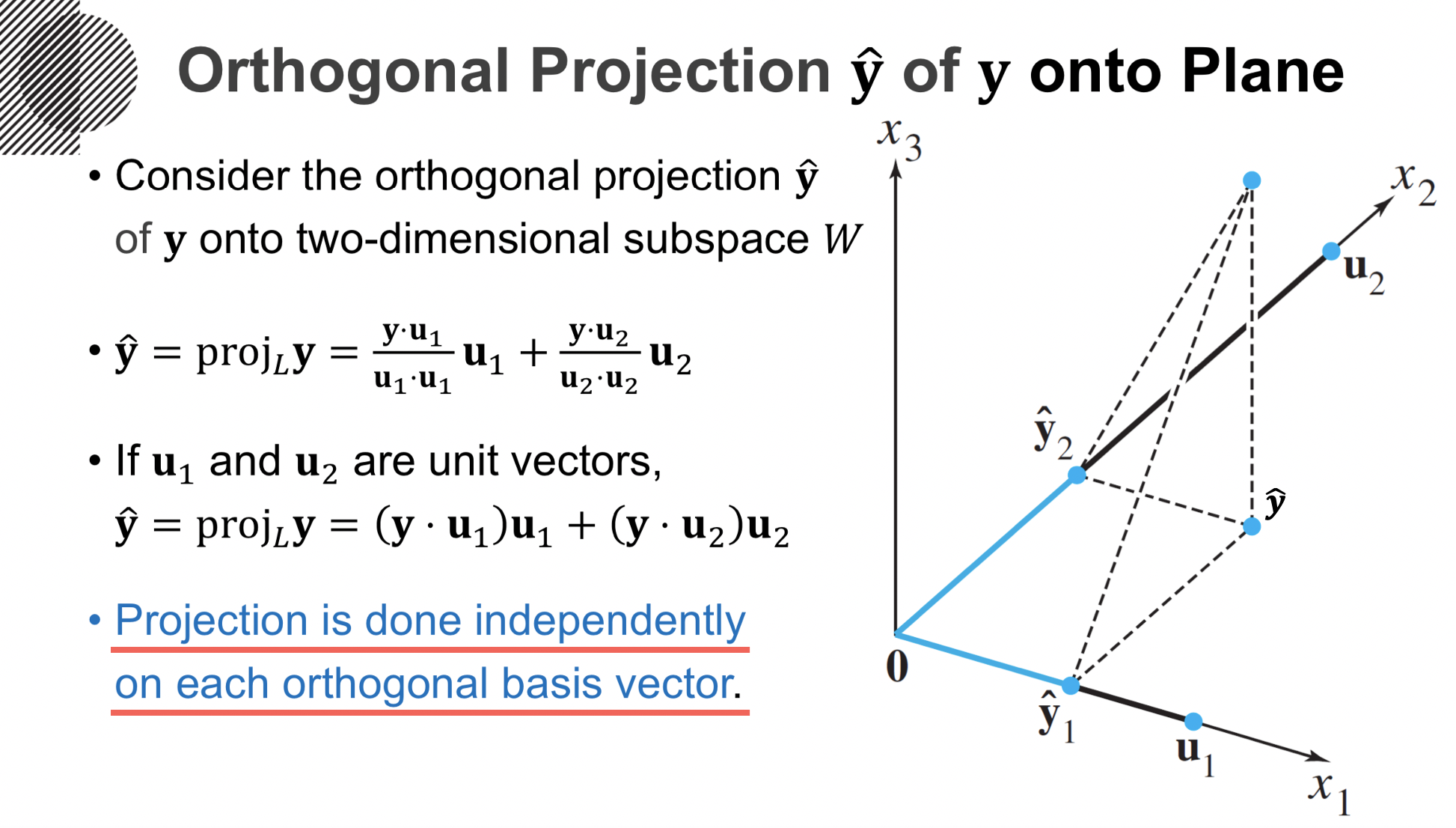
If $Q^T Q = I$, then $(Q^T Q)^{-1} = I^{-1} = I$. The formula becomes: $$ P = Q (I) Q^T = QQ^T $$

This is a much cleaner and more elegant formula. The projection of $b$ onto the subspace spanned by orthonormal columns $Q$ is simply $p = Q Q^{T} b$ . This has a beautiful interpretation: projecting onto an orthonormal basis is equivalent to summing the individual projections onto each basis vector.

This image shows the projection of a vector **y** onto a plane W spanned by two orthogonal vectors **u₁** and **u₂**. The total projection **ŷ** is the vector sum of the individual projections onto each basis vector, **ŷ₁** and **ŷ₂**. This works because the basis vectors are orthogonal.

Conclusion

In this lesson, we have derived one of the most fundamental tools in linear algebra: the orthogonal projection. By starting with the simple geometry of a right angle, we built up a complete algebraic solution for finding the closest point in any subspace to an external vector.

Key Takeaways:

Core Principle: The vector connecting a point to its orthogonal projection onto a subspace is orthogonal to that subspace.
The Normal Equation: This geometric principle gives rise to the algebraic equation $A^{T} A x^= A^{T} b$ , which finds the coefficients of the projection.
General Projection Matrix: For a subspace defined by the columns of a matrix $A$ , the projection matrix is $P = A (A^{T} A)^{- 1} A^{T}$ .
Orthonormal Simplification: If the basis for the subspace is orthonormal (columns of $Q$ ), the projection matrix simplifies to $P = Q Q^{T}$ .

This concludes our core study of linear algebra. The normal equation you derived today is not just an abstract concept; it is the solution to Ordinary Least Squares. In our next module on calculus, we will develop the tools (gradients and derivatives) to re-derive this same solution from an optimization perspective, completing the bridge from geometry to the language of machine learning.