PCA and Covariance Matrix Eigendecomposition

Introduction

In our previous lessons, we've built a strong geometric foundation in linear algebra, culminating in understanding projections and decompositions like SVD. We saw how these tools allow us to find optimal approximations and transform data into more revealing coordinate systems. Today, we'll explore a powerful application of these ideas: Principal Component Analysis (PCA).

This lesson serves as a capstone for our linear algebra module and a bridge to machine learning. PCA is a cornerstone of classical data analysis, used to simplify complex, high-dimensional datasets. For your goal of mastering both classical and modern AI, understanding PCA is crucial, as it represents the linear, geometric ancestor to non-linear dimensionality reduction techniques like the autoencoders we will encounter in deep learning.

Our objective is to understand PCA's core purpose—finding the most meaningful directions in a dataset—and to establish its fundamental identity: PCA is achieved by performing an eigendecomposition on the data's covariance matrix.

The Goal of PCA: Finding a Better Basis

Imagine you are working with a dataset from a physics simulation or a 3D scanner. You might have hundreds or even thousands of measurements for each data point. It's likely that many of these measurements are correlated or redundant. For instance, two nearby sensors might record very similar temperature values. The goal of dimensionality reduction is to find a more compact representation of this data, capturing the "essence" while discarding redundancy and noise.

PCA provides a formal, non-parametric way to do this. It aims to find a new coordinate system, a new basis, for the data. The key idea is that this new basis should be chosen so that the axes point in the directions of maximum variance in the data.

To get an intuitive feel for this, let's watch a short video that explains the motivation behind PCA.

As the video suggests, PCA constructs new axes (principal components) by combining the original ones. These new axes are ranked by importance, where importance is measured by variance. The first principal component is the direction in which the data is most spread out. The second principal component is the direction of most variance in the data orthogonal to the first, and so on. This creates a new, hierarchical, and data-driven basis.

Quantifying Relationships: The Covariance Matrix

To formalize the idea of finding directions of maximal variance, we first need a tool to quantify the relationships between all the different features (dimensions) in our dataset. This tool is the covariance matrix.

Let's assume we have a dataset represented by a matrix $X$, where each row is a data sample and each column is a different feature. Before we proceed, we must perform a crucial preprocessing step: mean-centering. For each feature column, we calculate its mean and subtract it from every entry in that column. This ensures our dataset is centered around the origin.

The covariance between two features measures how they vary together.

• A large positive covariance means that when one feature's value is high, the other's tends to be high as well.
• A large negative covariance means they are inversely related.
• A covariance near zero suggests they are uncorrelated.

The covariance matrix, which we'll denote as $C_X$, is a square, symmetric matrix where:

• The entry $C_X(i,i)$ on the diagonal is the variance of the $i$-th feature.
• The off-diagonal entry $C_X(i,j)$ is the covariance between the $i$-th and $j$-th features.

If our $N\times m$ data matrix $X$ is already mean-centered, its sample covariance matrix is defined as:

$$C_X=\frac{1}{N-1}{X}^{T}X$$

Our goal in PCA is to find a new basis where the features are uncorrelated.

Question: If we transform our data into a new representation where all features are uncorrelated, what would the covariance matrix of this new data look like?

Answer

If all features are uncorrelated, then all the off-diagonal elements of the covariance matrix, which represent the covariances between different features, must be zero. Therefore, the covariance matrix would be a **diagonal matrix**.

This insight is the key. The entire problem of PCA reduces to finding a rotation (an orthogonal transformation) that diagonalizes the covariance matrix.

For a more thorough walkthrough of the concepts of variance, redundancy, and the construction of the covariance matrix, the following reading is highly recommended.

The Solution: Eigendecomposition of the Covariance Matrix

We have now framed our problem: find an orthogonal transformation matrix $P$ that transforms our data $X$ into new data $Y$ such that the covariance matrix of $Y$, $C_Y$, is diagonal.

Let our transformation be a rotation defined by an orthogonal matrix $Q$. The transformed data is $X^{\prime }=XQ$. Let's see what the new covariance matrix $C^{\prime }$ becomes:

$$C^{\prime }=\frac{1}{N-1}(X^{\prime }{)}^T{X}^{\prime }=\frac{1}{N-1}(XQ{)}^T(XQ)$$

Using the property $(AB{)}^T=B^T{A}^T$, we get:

$$C^{\prime }=\frac{1}{N-1}(Q^T{X}^T)(XQ)=Q^T\left(\frac{1}{N-1}{X}^{T}X\right)Q$$

Recognizing the term in the middle as the original covariance matrix $C_X$, we have:

$$C^{\prime }=Q^T{C}_{X}Q$$

We want $C^{\prime }$ to be a diagonal matrix, let's call it $\Lambda$. So the equation we need to solve is:

$$\Lambda =Q^T{C}_{X}Q$$

If we multiply from the left by $Q$, and recall that for an orthogonal matrix $Q^T=Q^{-1}$, we get:

$$Q\Lambda =Q{Q}^T{C}_{X}Q=(Q{Q}^{-1})C_{X}Q=I{C}_{X}Q=C_{X}Q$$

So we arrive at:

$$C_{X}Q=Q\Lambda$$

This is precisely the eigenvalue equation for the matrix $C_X$!

This is the central result of PCA.

• The columns of the matrix $Q$ are the eigenvectors of the covariance matrix $C_X$. These eigenvectors are the principal components—the axes of our new, optimal basis.
• The diagonal matrix $\Lambda$ contains the eigenvalues of $C_X$. Each eigenvalue ${\lambda }_i$ corresponds to the variance of the data projected onto its associated eigenvector $q_i$.

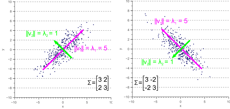
The magnitude of the eigenvalues tells us the "importance" of each principal component. The eigenvector with the largest eigenvalue is the first principal component, capturing the direction of maximum variance. The eigenvector with the second-largest eigenvalue is the second principal component, and so on.

The image below provides a perfect visual summary. It shows two different 2D datasets (scatter plots). The principal components are the eigenvectors of the covariance matrix ($\Sigma$), shown as the magenta and green vectors. The length of the vectors, representing the variance, corresponds to the eigenvalues (${\lambda }_1,{\lambda }_2$).

To see this derivation presented from a slightly different but equally valid perspective, you can consult the following resource.

The PCA Algorithm and Dimensionality Reduction

We can now summarize the entire PCA process as a concrete algorithm:

1. Given an $N\times m$ data matrix $X$, where $N$ is the number of samples and $m$ is the number of features.
2. Mean-center the data: For each feature (column), subtract its mean.
3. Compute the covariance matrix: $C_X=\frac{1}{N-1}{X}^{T}X$.
4. Compute the eigendecomposition of $C_X$: Find the eigenvalues ${\lambda }_1,\dots ,{\lambda }_m$ and corresponding eigenvectors $q_1,\dots ,q_m$.
5. Sort the components: Order the eigenvectors according to their corresponding eigenvalues, from largest to smallest. The sorted eigenvectors form the columns of your transformation matrix $Q$.
6. Transform the data: The new data in the principal component basis is given by $X^{\prime }=XQ$.

So, how does this lead to dimensionality reduction? We simply decide to keep only the top $k$ principal components, where $k<m$. By projecting our data onto the subspace spanned by these first $k$ eigenvectors, we create a $k$-dimensional representation that preserves the maximum possible variance from the original data. The amount of total variance captured by the first $k$ components is given by the ratio:

$$\text{Variance Explained}=\frac{{\sum }_{i=1}^k{\lambda }_i}{{\sum }_{j=1}^m{\lambda }_j}$$

A common practice is to choose $k$ such that you retain a desired percentage of the variance, for example, 95% or 99%.

This process of selecting the most important components based on their associated variance is explained well in the following video.

Conclusion

In this reference lesson, we've connected the abstract concepts of eigendecomposition to the practical task of dimensionality reduction. PCA provides a powerful, principled method for simplifying complex data by finding a new basis that reveals its underlying structure.

Key Takeaways:

• PCA Goal: To find a new orthogonal basis for a dataset where the axes align with the directions of maximum variance.
• Core Identity: This goal is accomplished by finding the eigenvectors of the data's covariance matrix.
• Principal Components: The eigenvectors of the covariance matrix are the principal components, which form the new basis vectors.
• Variance Explained: The corresponding eigenvalues quantify the variance along each principal component, allowing us to rank them by importance and perform dimensionality reduction by keeping only the most significant ones.

PCA is a purely linear technique; it discovers the best flat subspace (a hyperplane) to project the data onto. This provides a crucial point of contrast for our future studies. When we get to deep learning, we will explore autoencoders, which can be understood as a non-linear generalization of PCA. Instead of finding a flat hyperplane, an autoencoder can learn a complex, curved, low-dimensional manifold that the data lies on, enabling far more powerful compression and representation.

This lesson concludes our module on linear algebra. You now have the geometric and algebraic tools needed to understand how data is represented and manipulated. In our next module, we will turn to Multivariable Calculus. We'll develop the concepts of derivatives and gradients, which are the language of change and optimization, and are essential for training any machine learning model.