SVD: Decomposing Linear Transformations

Introduction

In our last lesson, we explored how eigendecomposition, $A=P\Lambda P^{-1}$, reveals the principal axes of a linear transformation. We saw that for matrices with a full set of eigenvectors, the transformation is fundamentally a simple scaling along these axes. However, this powerful picture has a limitation: it doesn't apply to all matrices. A shear transformation, for example, doesn't have enough eigenvectors to form a basis, and rectangular matrices don't have eigenvectors at all.

This raises a crucial question: Is there a more general geometric decomposition that works for any matrix? Can we find an intuitive geometric meaning—a set of principal axes—for transformations like shears, or even for maps between different dimensions (e.g., from ${\mathbb{R}}^3$ to ${\mathbb{R}}^2$)?

The answer is a resounding yes, and it is given by the Singular Value Decomposition (SVD). This lesson will focus on developing the powerful geometric intuition behind SVD. We will see that any linear transformation, no matter how complex, can be broken down into a sequence of three fundamental operations: a rotation, a scaling, and another rotation.

The Universal Geometric Recipe: Rotation, Scaling, Rotation

The Singular Value Decomposition states that any $m\times n$ matrix $A$ can be factored into the product of three other matrices:

$$A=U\Sigma V^T$$

where:

• $V^T$ is an $n\times n$ orthogonal matrix. Geometrically, it represents a rotation (and possibly a reflection) in the input space ${\mathbb{R}}^n$.
• $\Sigma$ (Sigma) is an $m\times n$ diagonal matrix. Its diagonal entries, ${\sigma }_1,{\sigma }_2,\dots$, are the singular values of $A$. Geometrically, this matrix performs a scaling along the new, rotated axes. If the dimensions $m$ and $n$ differ, it also handles the change in dimension.
• $U$ is an $m\times m$ orthogonal matrix. It represents a final rotation in the output space ${\mathbb{R}}^m$.

The profound insight of SVD is that even the most complex-looking transformations, like shears, are just simple axis-aligned scaling operations viewed from a "tilted" perspective. SVD finds the perfect "un-tilting" and "re-tilting" rotations to reveal this simple scaling at the core.

Deconstructing a Shear Transformation

Let's use a shear transformation as a test case. As we saw, a shear is tricky for eigendecomposition. However, SVD handles it with ease. The key idea is that we can break down the shear into a sequence of simpler, more intuitive steps.

The following article provides a superb visual and textual explanation for this exact process.

As you saw, the process unfolds in three steps:

1. First Rotation ($V^T$): This initial rotation aligns a specific set of orthogonal vectors in the input space with the standard coordinate axes ($e_1,e_2,\dots$). These aren't just any vectors; they are the special directions that will remain orthogonal after being transformed by $A$. These are called the right singular vectors and form the columns of $V$.
2. Scaling ($\Sigma$): With the input space correctly aligned, the transformation becomes a simple scaling. The space is stretched or squished along each axis. The amount of scaling on each axis is given by the corresponding singular value ${\sigma }_i$. If the matrix is rectangular, this step also adds or removes dimensions.
3. Second Rotation ($U$): The scaled vectors now lie along the axes of the output space. This final rotation moves them into their final orientation. The destination axes for this rotation are the left singular vectors, which form the columns of $U$.

The Canonical Visualization: Transforming a Sphere

Perhaps the most fundamental geometric interpretation of SVD is its effect on a unit sphere (or a unit circle in 2D). For any matrix $A$, the transformation $A\vec{x}$ maps the unit sphere in the input space to an ellipsoid in the output space.

SVD reveals the geometry of this transformation:

• The right singular vectors (${\vec{v}}_i$, columns of $V$) are the orthogonal vectors on the input unit sphere that become the principal axes of the output ellipsoid.
• The left singular vectors (${\vec{u}}_i$, columns of $U$) are the orthogonal principal axes of the output ellipsoid.
• The singular values (${\sigma }_i$) are the lengths of these principal axes.

The following article develops this idea from first principles, starting with a simple square.

This circle-to-ellipse mapping is the heart of SVD's geometry. The entire complex deformation of space caused by $A$ is captured by identifying the principal axes of this resulting ellipsoid ($U$), determining how much they were stretched ($\Sigma$), and finding which input vectors gave rise to them ($V$).

Putting It All Together: A Visual Summary

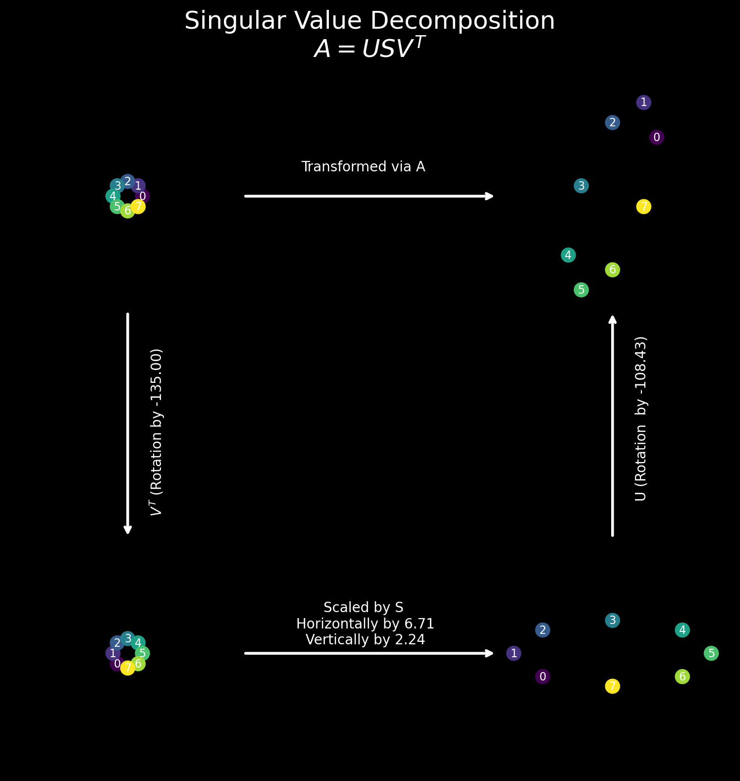
We have seen the components of SVD in action. Now, let's watch a video that animates the entire process, showing how the three operations compose to produce the final transformation.

The following image provides a static summary of the two equivalent paths to transform a set of points, as shown in the video.

Bridging Geometry and Algebra

We have established the geometric picture. Now, let's briefly connect this intuition back to the algebraic formulation.

We said that the right singular vectors ${\vec{v}}_i$ are mapped to the axes of the output ellipse, which are the left singular vectors ${\vec{u}}_i$ scaled by the singular values ${\sigma }_i$.

Question: Based on this description, how would you write an equation that relates a single vector ${\vec{v}}_i$ to its transformed counterpart using the matrix $A$, the vector ${\vec{u}}_i$, and the scalar ${\sigma }_i$?

Answer

The transformation of $\vec{v}_i$ by $A$ results in the vector $\vec{u}_i$ scaled by $\sigma_i$. So, the equation is: $$ A\vec{v}_i = \sigma_i \vec{u}_i $$

This simple equation holds for all $i=1,\dots ,n$. We can stack these vector equations side-by-side into a single matrix equation:

$$A[{\vec{v}}_1|{\vec{v}}_2|\dots |{\vec{v}}_n]=[{\sigma }_1{\vec{u}}_1|{\sigma }_2{\vec{u}}_2|\dots |{\sigma }_n{\vec{u}}_n]$$

This can be rewritten more compactly. The left side is simply $AV$. The right side can be factored into the product of the matrix of left singular vectors $U$ and the diagonal matrix of singular values $\Sigma$. This gives us:

$$AV=U\Sigma$$

Finally, since $V$ is an orthogonal matrix, its inverse is its transpose ($V^{-1}=V^T$). Right-multiplying by $V^T$ gives us the familiar form of the SVD:

$$A=U\Sigma V^T$$

This shows how the geometric picture of mapping orthogonal input vectors to orthogonal output vectors directly leads to the algebraic decomposition.

Conclusion

In this lesson, we established the geometric foundation of the Singular Value Decomposition. Unlike eigendecomposition, which is limited to certain square matrices, SVD provides a universal and intuitive way to understand any linear transformation.

Key Takeaways:

• Universal Decomposition: Any $m\times n$ matrix $A$ can be decomposed into $A=U\Sigma V^T$.
• Geometric Meaning: This decomposition represents any linear transformation as a sequence of three simpler operations: an initial rotation ($V^T$), an axis-aligned scaling ($\Sigma$), and a final rotation ($U$).
• Sphere to Ellipsoid: SVD formalizes the idea that any linear map transforms a unit sphere into an ellipsoid. The singular vectors ($U$ and $V$) define the principal axes of this mapping, and the singular values ($\Sigma$) define the extent of stretching along those axes.

We now have a solid intuition for what SVD is and why it's so fundamental. But how do we actually find the matrices $U$, $\Sigma$, and $V$ for a given matrix $A$? In our next lesson, we will answer this question by deriving the full algebraic procedure for computing the SVD, revealing a deep and elegant connection back to the eigendecomposition of the symmetric matrices $A^{T}A$ and $A{A}^T$.