Geometric Interpretation of Eigendecomposition

Recommended resources

The freely available resources this lesson will direct you to.

Introduction

In our previous lesson, we developed the algebraic machinery to compute eigenvalues and eigenvectors. By solving the characteristic equation $det (A - λ I) = 0$ , we could find the eigenvalues $λ$ of a matrix $A$ , and for each $λ$ , we found its corresponding eigenvectors $v$ by finding the null space of $(A - λ I)$ .

While this procedure is effective, it doesn't immediately convey why these values are so important. This lesson moves from the "how" to the "why" by focusing on the geometric meaning of eigendecomposition. Our goal is to interpret this process as identifying the principal axes of a linear transformation—the intrinsic directions along which the transformation acts as a simple scaling. Understanding this geometry is not just an academic exercise; it is the foundation for many advanced techniques in graphics, physics, and machine learning, including Principal Component Analysis (PCA), which we will touch upon today.

The Geometry of Invariant Directions

Recall the defining equation: $A v = λ v$ . Geometrically, this means that an eigenvector $v$ of a matrix $A$ is a vector whose direction is left unchanged, or invariant, by the transformation $A$ . The vector $A v$ lies on the same line (the span) as $v$ . The eigenvalue $λ$ is simply the factor by which the eigenvector is stretched ( $∣ λ ∣ > 1$ ), shrunk ( $∣ λ ∣ < 1$ ), or flipped ( $λ < 0$ ).

Most vectors, when transformed, are both scaled and rotated. Eigenvectors are special because they are only scaled. They define the axes of the transformation where the behavior is purest.

To see this in action, let's watch a short segment that visualizes how eigenvectors behave during a transformation compared to other vectors.

What is an Eigenvector?

The video "What is an Eigenvector?" from Leios Labs provides an excellent 3D visualization of this concept.

Watch the segment from this timestamp. Observe the deforming grid. While most points are moved and rotated, focus on the lines that only stretch or shrink without changing their orientation. These are the directions of the eigenvectors.

A classic way to visualize a 2D transformation is to see its effect on a unit circle. A linear transformation maps a unit circle to an ellipse. The eigenvectors of the transformation matrix point along the major and minor axes of this resulting ellipse.

This diagram illustrates a linear transformation A mapping a unit circle (blue, representing input vectors x) to an ellipse (red, representing output vectors Ax). The eigenvectors v1 and v2 align perfectly with the principal axes of the resulting ellipse.

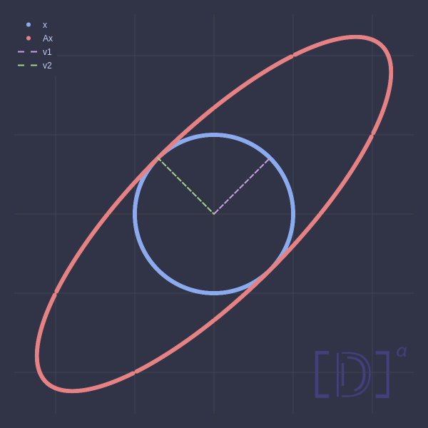
Looking at this image, the transformation stretches space more in the direction of one eigenvector and less in the direction of the other. The eigenvalues would represent the magnitude of this stretch along each of these principal axes.

Special Transformations and Their Principal Axes

We can build a strong geometric intuition by analyzing the eigenvectors of transformations you're already familiar with from computer graphics.

Projection

Consider a matrix $P$ that projects every vector in $R^{2}$ onto the x-axis.

Any vector already on the x-axis, like $v = (c 0)$ , is unchanged. Thus, $P v = v$ . These vectors are eigenvectors with eigenvalue $λ = 1$ . The entire x-axis is an eigenspace.
Any vector on the y-axis, like $v = (0 c)$ , is projected to the origin. Thus, $P v = 0 = 0 \cdot v$ . These vectors are eigenvectors with eigenvalue $λ = 0$ . The entire y-axis is the other eigenspace.

The principal axes are clear: the space being projected onto (kept, $λ = 1$ ) and the space being projected away (destroyed, $λ = 0$ ).

Reflection

Now consider a matrix $R$ that reflects every vector in $R^{2}$ across the x-axis.

A vector on the x-axis is unchanged by the reflection. It's an eigenvector with $λ = 1$ .
A vector on the y-axis is flipped to point in the opposite direction. It's an eigenvector with $λ = - 1$ .

Once again, the principal axes are the line of reflection itself and the direction perpendicular to it.

The following text from Professor Gilbert Strang's textbook formalizes these exact examples.

Chapter 6 Eigenvalues and Eigenvectors

This excerpt from Strang's Introduction to Linear Algebra provides concise explanations for the eigenvalues of projection and reflection matrices.

Please read the section on "Example 2" and "Example 3" here. Note how the geometric action of the matrix directly reveals its eigenvalues and eigenvectors without needing the characteristic equation.

Rotation

What about a 90-degree rotation in 2D? A moment's thought should convince you that no non-zero real vector keeps its direction after a 90-degree rotation. Every vector is moved off its own span.

Question: If there are no real eigenvectors, what does this imply about the roots of the characteristic equation for a 2D rotation matrix?

Answer

It implies that the characteristic equation has no real roots. The eigenvalues must be complex numbers. For a 90-degree rotation, the eigenvalues are $i$ and $-i$.

This is a profound link between geometry and algebra. The geometric absence of invariant directions manifests as the algebraic absence of real eigenvalues.

However, in 3D, the story is different. Any rotation in 3D space must occur around an axis of rotation. Any vector lying on this axis is an eigenvector with eigenvalue $λ = 1$ , as it is not changed by the rotation. This is a critical concept in 3D graphics and robotics for representing orientations and angular velocities.

Eigenvectors and eigenvalues | Chapter 14, Essence of linear algebra

The 3Blue1Brown video on Eigenvectors and Eigenvalues explains this beautifully.

First, watch the segment on 3D rotation from this point to see how the eigenvector defines the axis of rotation. Then, watch the segment on 2D rotation from this part to see how it leads to complex eigenvalues.

Eigendecomposition: Changing to a Better Basis

We can formalize this geometric intuition. If an $n \times n$ matrix $A$ has $n$ linearly independent eigenvectors, we can use them to form a new basis for $R^{n}$ . This basis is called the eigenbasis.

Let the eigenvectors be $v_{1}, v_{2}, \dots, v_{n}$ with corresponding eigenvalues $λ_{1}, λ_{2}, \dots, λ_{n}$ . We can assemble these into two matrices:

$P$ : A matrix whose columns are the eigenvectors: $P = [v_{1} ∣ v_{2} ∣ \dots ∣ v_{n}]$ .
$Λ$ (Lambda): A diagonal matrix with the eigenvalues on the diagonal: $Λ = λ_{1} 0 ⋮ 0 0 λ_{2} ⋮ 0 \dots \dots ⋱ \dots 00 ⋮ λ_{n}$

The set of all eigenvalue equations $A v_{i} = λ_{i} v_{i}$ can be written compactly in matrix form as:

A P = P Λ

If the eigenvectors are linearly independent, then $P$ is invertible, and we can write:

A = P Λ P^{- 1}

This is the eigendecomposition or diagonalization of matrix $A$ .

This equation gives us a recipe for understanding the transformation $A$ :

$P^{- 1}$ : Apply $P^{- 1}$ to a vector $x$ . This is a change of basis that re-expresses $x$ in the coordinates of the eigenbasis.
$Λ$ : Multiply by the diagonal matrix $Λ$ . In the eigenbasis, the transformation is a simple scaling along each basis vector (the eigenvectors). The scaling factors are the eigenvalues.
$P$ : Apply $P$ to the result. This is another change of basis that converts the vector back to the standard coordinate system.

In essence, eigendecomposition reveals that every transformation with a full set of eigenvectors is just a simple scaling along its principal axes. The complexity of the matrix $A$ is just a result of viewing this simple scaling from the perspective of the "wrong" (i.e., standard) basis.

The following article provides a fantastic visual walkthrough of this exact idea.

Eigenvalues and eigenvectors

This blog post by Peter Bloem uses domain coloring with the Mona Lisa to provide a clear, intuitive explanation of eigendecomposition as a change of basis, scaling, and change of basis back.

First, read the section What are eigenvectors? to solidify the concept of eigenvectors as invariant directions. Then, carefully study the next section, which explains eigendecomposition as three steps: rotation, scaling, and inverse rotation. Pay close attention to the mona-steps.svg image and the derivation of the formula \bc{A} = \rc{P}\bc{\D}\rc{\P}^{-1}. (Note: The blog uses \bc{D} where we use \Lambda, a common notational difference).

Application: Principal Axes of Data

So far, we have viewed matrices as transformations. But in machine learning, we often work with matrices that represent data. One of the most important applications of eigendecomposition is Principal Component Analysis (PCA), a technique for dimensionality reduction.

Imagine you have a cloud of data points, like measurements of many different properties of a system. PCA finds the "principal axes" of this data cloud—the directions in which the data varies the most.

How does it do this?

The data is organized into a data matrix $X$ .
We compute the covariance matrix of the data, typically denoted $S$ or $Σ$ . This matrix tells us how different features (columns of $X$ ) vary together. For mean-centered data, it's calculated as $S = \frac{1}{N} X^{T} X$ .
We then find the eigenvectors and eigenvalues of this covariance matrix $S$ .

The geometric interpretation is powerful:

The eigenvectors of the covariance matrix are the principal components of the data. They are orthogonal vectors that point in the directions of maximum variance.
The eigenvalues tell us the amount of variance along each of these principal directions.

The first principal component (the eigenvector with the largest eigenvalue) is the single axis that captures the most information about the data. The second principal component is the orthogonal axis that captures the next most, and so on. By projecting the data onto the first few principal components, we can reduce its dimensionality while losing minimal information.

The blog post you just read builds up to this exact conclusion.

Eigenvalues and eigenvectors

This reading connects the geometric intuition of eigenvectors as principal axes of a transformation to their role as principal components of a dataset.

Start at the section Eigenvectors of which matrix?, which introduces the covariance matrix. Then, read the section Quadratic forms to see how the eigenvectors of the covariance matrix define an ellipsoid that encapsulates the data. Finally, read the section Why is PCA optimal?, which formally proves that the first principal component is the eigenvector with the largest eigenvalue—the direction of maximum variance.

Conclusion

In this lesson, we moved beyond mere calculation to uncover the rich geometric meaning behind eigenvalues and eigenvectors. They are not just arbitrary numbers but are intimately tied to the fundamental structure of a linear transformation.

Key Takeaways:

Principal Axes: Eigenvectors represent the invariant directions of a linear transformation—its principal axes. Along these axes, the transformation acts as a simple scaling.
Geometric Interpretation of $λ$ : The eigenvalue $λ$ is the scaling factor along the corresponding eigenvector's axis. The sign of $λ$ indicates whether the direction is preserved or flipped, and its magnitude indicates stretching or shrinking.
Eigendecomposition ( $A = P Λ P^{- 1}$ ): This decomposition reveals that any transformation with a full set of eigenvectors is fundamentally a simple scaling ( $Λ$ ) viewed in a different coordinate system (the eigenbasis defined by $P$ ).
Application to PCA: In data analysis, the eigenvectors of the covariance matrix represent the principal components of the data—the orthogonal axes of greatest variance. This provides a direct and powerful application of the "principal axes" concept.

In our next lesson, we will explore the Singular Value Decomposition (SVD). SVD is even more general and powerful than eigendecomposition; it can be applied to any matrix, not just square ones. It decomposes a transformation into a sequence of rotation, scaling, and another rotation, and it forms the mathematical backbone of countless algorithms in computer graphics, machine learning, and scientific computing.