Bias-Variance Tradeoff: Model Complexity & Regularization

In our last lesson, we delved into the mechanics of L1 and L2 regularization, understanding them as constrained optimization problems that prevent our models from becoming excessively complex. We saw how they shrink model weights, and in Lasso's case, even perform feature selection. You now have the "how." Today, we will explore the fundamental "why."

This lesson formalizes the intuition behind regularization by introducing one of the most central concepts in machine learning: the bias-variance tradeoff. Our learning outcome is to explain the bias-variance tradeoff and its relationship to model complexity and regularization. We will mathematically decompose a model's generalization error and see that a model can be wrong for two very different reasons: it can be too simple (high bias) or too sensitive (high variance). Understanding this tradeoff is what elevates a practitioner from simply applying algorithms to truly diagnosing and engineering model performance.

The Anatomy of Error

Imagine you are an archer aiming at a target. Your performance can be poor in two distinct ways. You might be consistently hitting the same spot, but far to the left of the bullseye. This is a systematic error, or bias. Alternatively, your shots might be scattered all over the target, centered on average around the bullseye, but individually imprecise. This is an error of inconsistency, or variance. A machine learning model's error behaves in much the same way.

The video below from Professor Kilian Weinberger's course at Cornell provides an excellent visual analogy using a dartboard and a rigorous derivation of this concept.

The Bias-Variance-Noise Decomposition

As the lecture demonstrated, the expected prediction error of a model at a given point $x$ can be rigorously decomposed into three components. Let's assume the true data-generating process is $y=f(x)+ϵ$, where $ϵ$ is random noise with zero mean and variance ${\sigma }_{ϵ}^2$. Our model, $\hat{f}(x)$, is trained on a specific dataset $D$.

The expected squared prediction error is:

Let's unpack each term:

• Bias²: This term measures the difference between the average prediction of our model (across all possible training sets) and the true underlying function $f(x)$. High bias means that, on average, our model's fundamental assumptions are wrong and it fails to capture the true relationship. This leads to underfitting. A simple linear model trying to fit a complex, parabolic trend is a classic example of a high-bias model. It is systematically incorrect.

• Variance: This term measures how much the model's prediction $\hat{f}(x)$ varies for different training datasets. High variance means the model is overly sensitive to the specific data it was trained on—it learns the noise, not just the signal. This leads to overfitting. A high-degree polynomial that wiggles to pass through every single training point is a high-variance model. Its predictions would change dramatically if trained on a slightly different set of points.

• Irreducible Error (Noise): This term is due to the inherent randomness in the data itself. No matter how good our model is, we can never predict the noise component $ϵ$. This error sets a theoretical lower bound on the performance of any model.

This decomposition is one of the most important theoretical results in machine learning. It tells us that our attempts to reduce error are a balancing act.

The Tradeoff and Model Complexity

The relationship between bias and variance is typically governed by model complexity.

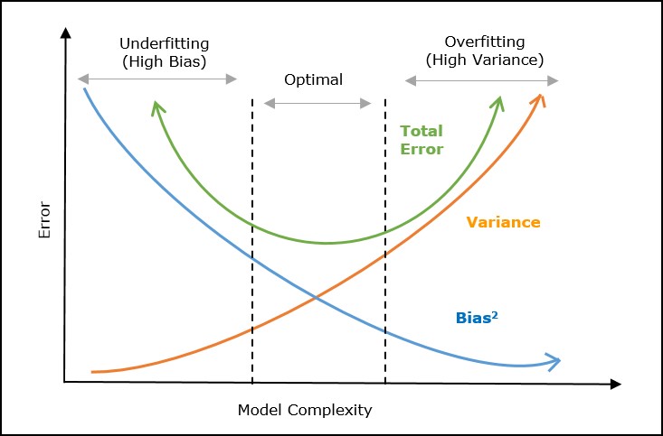
Let's analyze the relationship shown in the graph:

• Low Complexity (Underfitting): On the left side, we have simple models (e.g., linear regression, or a decision tree with a very small depth). These models have high bias because they are not flexible enough to capture the underlying structure of the data. However, they have low variance because they are stable; changing the training data a little won't drastically change the simple line they fit.
• High Complexity (Overfitting): On the right side, we have complex models (e.g., a high-degree polynomial, or a very deep decision tree). These models have low bias because they are flexible enough to fit the training data almost perfectly. But this flexibility comes at the cost of high variance. They are exquisitely tuned to the training data, including its noise, and will not generalize well to unseen data.
• The "Sweet Spot": In the middle, there is an optimal level of complexity that minimizes the total error. This is the goal of model selection.

Regularization's Role in the Tradeoff

This brings us back to our last lesson on L1 and L2 regularization. We can now understand regularization in the context of this tradeoff.

Regularization is a technique to control model complexity, thereby navigating the bias-variance tradeoff.

When we add a penalty term like $\lambda ||\mathbf{w}|{|}_2^2$ or $\lambda ||\mathbf{w}|{|}_1$ to our loss function, we are constraining the model's capacity. We are preventing the weights from becoming too large, which in turn prevents the model from fitting the training data too precisely.

In the language of the tradeoff:

• Regularization intentionally increases the bias of the model. We are forcing it to be "simpler" than it would otherwise be, so its average prediction will be slightly further from the true function.
• In exchange, regularization dramatically reduces the variance. By constraining the weights, the model becomes less sensitive to the noise in any particular training set. The resulting function is smoother and more stable.

The regularization parameter $\lambda$ directly controls this tradeoff. A small $\lambda$ leads to a complex model with low bias and high variance. A large $\lambda$ leads to a simple model with high bias and low variance. Our goal is to tune $\lambda$ (often via cross-validation, a topic for our next module) to find the point that minimizes the total error.

The following article provides a superb, detailed walkthrough of the entire decomposition and its implications.

Beyond the Classical View: Double Descent

For many years, the U-shaped curve was considered the complete story. However, in the modern era of extremely large models like deep neural networks, a fascinating phenomenon called double descent has been observed.

In this regime, as model complexity increases past the point of "interpolation" (where it can perfectly fit the training data), the test error, after peaking, can start to decrease again. This happens in "overparameterized" models where the number of parameters is much larger than the number of data points.

This discovery doesn't invalidate the bias-variance framework but extends it. It suggests that in these highly overparameterized regimes, the optimization algorithms themselves (like gradient descent) induce a form of implicit regularization that continues to reduce variance even as complexity soars. Given your interest in AI system design, it is crucial to know that for state-of-the-art models, the "sweet spot" might not be at the bottom of the classical "U," but far to the right in this second descent.

Conclusion

Today, we've moved from the "how" of regularization to the fundamental "why." The bias-variance tradeoff provides the theoretical language to describe the central challenge of supervised learning: building a model that is complex enough to capture the true signal without being so complex that it mistakes noise for signal.

Key Takeaways:

• A model's expected generalization error can be decomposed into three components: Bias², Variance, and Irreducible Error.
• Bias is the error from a model's incorrect assumptions, leading to underfitting.
• Variance is the error from a model's sensitivity to the training data, leading to overfitting.
• Model Complexity is the primary driver of the tradeoff: simple models have high bias and low variance, while complex models have low bias and high variance.
• Regularization is our explicit tool for controlling this tradeoff. It increases bias to decrease variance, aiming to find the optimal balance that minimizes total error.

In our next lesson, we will make this concrete by examining polynomial regression. We'll see firsthand how increasing the degree of a polynomial increases model complexity, and how this directly creates the risk of high variance (overfitting) that we've discussed today.