Regularization: Lasso and Ridge as Constrained Optimization

Recommended resources

The freely available resources this lesson will direct you to.

Welcome to our next lesson. In our previous discussion, we explored the optimization landscape, distinguishing between the predictable, "bowl-shaped" world of convex problems and the rugged, unpredictable terrain of non-convex ones. We now have a solid understanding that for many fundamental models, gradient descent will reliably find the single best solution that minimizes the in-sample error.

However, minimizing in-sample error is only a means to an end. Our true goal is generalization—performance on new, unseen data. An overzealous optimization that perfectly fits the training data often learns the noise along with the signal, a phenomenon known as overfitting. To combat this, we must deliberately constrain our models. This lesson introduces regularization, a powerful and principled technique for doing just that.

Our learning outcome is to derive L1 (Lasso) and L2 (Ridge) regularization as constrained optimization problems and explain their effects on model weights. We will see how, by adding a penalty term to our loss function, we transform the optimization problem itself. We move from simply asking "What weights minimize the training error?" to "What is the 'simplest' set of weights that still explains the data well?"

Regularization: Putting the Brakes on Optimization

In essence, regularization introduces a "penalty" for model complexity. If our model is a linear or polynomial regression, complexity is often synonymous with large coefficient values, which allow the model to bend and twist sharply to fit every data point. By penalizing large weights, we encourage the learning algorithm to find smoother, simpler solutions that are more likely to capture the underlying trend.

This is not a random heuristic; it is a mathematically grounded approach to improving generalization. The Caltech lecture by Professor Yaser Abu-Mostafa provides an excellent framing of this concept.

Lecture 12 - Regularization

This video introduces the concept of regularization as a 'cure' for overfitting, framing it as both a mathematical and heuristic technique.

First, watch the introduction to regularization from the start. The professor discusses the two main perspectives on regularization: a formal mathematical derivation and a more heuristic approach of "handicapping" the minimization. Next, watch the segment that frames regularization as a constrained optimization problem, from this point. This section introduces the core idea we will build upon: minimizing the in-sample error subject to a budget on the magnitude of the weights.

The general form of a regularized objective function is:

J_{r e g} (w) = Loss (data ∣ w) + λ \cdot Penalty (w)

Here, $λ$ is the regularization parameter, a hyperparameter that controls the strength of the penalty. A larger $λ$ enforces a stronger penalty, pushing the model towards greater simplicity. The specific form of the penalty term defines the type of regularization. We will now explore the two most common forms: L2 and L1.

L2 Regularization: Ridge Regression

L2 regularization, also known as Ridge Regression when applied to linear regression, penalizes the sum of the squared magnitudes of the weights. This is the squared L2-norm of the weight vector, $∣∣ w ∣ ∣_{2}^{2}$ .

The objective function becomes:

J_{r i d g e} (w) = MSE (w) + λ ∣∣ w ∣ ∣_{2}^{2} = \frac{1}{N} i = 1 \sum N (y_{i} - w^{T} x_{i})^{2} + λ j = 1 \sum d w_{j}^{2}

Derivation as a Constrained Problem

This formulation is equivalent to solving a constrained optimization problem. We seek to minimize the original loss function (e.g., MSE) subject to the constraint that the squared L2-norm of the weights does not exceed a certain budget, $C$ .

w min MSE (w) subject to ∣∣ w ∣ ∣_{2}^{2} \leq C

Using the method of Lagrange multipliers, we can convert this constrained problem into the unconstrained form shown above. The regularization parameter $λ$ is the Lagrange multiplier, which has an inverse relationship with the budget $C$ : a smaller budget $C$ (a tighter constraint) corresponds to a larger penalty $λ$ .

The Caltech lecture provides a brilliant pictorial proof of this equivalence, which is far more intuitive than a purely algebraic derivation.

Lecture 12 - Regularization

This segment walks through the geometric interpretation of converting the L2-constrained problem into its unconstrained, "augmented error" form.

Watch the derivation from this key section. The visual shows the contours of the error function (ellipses) and the constraint region (a circle). The solution, w_reg, must lie where the smallest possible error contour touches the constraint boundary. At this point of tangency, the gradient of the loss function is anti-parallel to the gradient of the constraint, which leads directly to the unconstrained formulation.

The Closed-Form Solution

A significant advantage of L2 regularization is that the new objective function remains convex and differentiable. Therefore, we can find a global minimum by taking the gradient with respect to $w$ , setting it to zero, and solving. This yields a closed-form solution for the Ridge Regression weights:

w_{r i d g e} = (X^{T} X + λ I)^{- 1} X^{T} y

Compare this to the Ordinary Least Squares solution: $w_{O L S} = (X^{T} X)^{- 1} X^{T} y$ . The addition of the $λ I$ term, the "ridge," has two important effects:

Guaranteed Invertibility: The matrix $X^{T} X$ might be singular or ill-conditioned, especially if features are highly correlated (multicollinearity). Adding a positive value $λ$ to the diagonal ensures the matrix is invertible.
Weight Shrinkage: As $λ$ increases, the $λ I$ term dominates, and the weights are "shrunk" towards zero. This effect is often called weight decay. However, the weights will approach zero asymptotically but will almost never become exactly zero.

The following resources provide the full analytical derivation and a probabilistic interpretation.

Understanding L1 and L2 regularization with analytical and ...

This article provides a detailed mathematical walkthrough for both L2 and L1 regularization.

First, read the section on the analytical derivation. This shows the step-by-step process of differentiating the Ridge objective function to arrive at the closed-form solution. Next, read the section on the probabilistic derivation. This demonstrates that minimizing the L2-regularized loss is equivalent to performing Maximum A Posteriori (MAP) estimation assuming a Gaussian prior distribution over the weights. This gives L2 regularization a strong Bayesian justification.

L1 Regularization: Lasso Regression

L1 regularization, or Lasso (Least Absolute Shrinkage and Selection Operator), penalizes the sum of the absolute values of the weights—the L1-norm, $∣∣ w ∣ ∣_{1}$ .

The objective function is:

J_{l a sso} (w) = MSE (w) + λ ∣∣ w ∣ ∣_{1} = \frac{1}{N} i = 1 \sum N (y_{i} - w^{T} x_{i})^{2} + λ j = 1 \sum d ∣ w_{j} ∣

This is equivalent to the constrained problem:

w min MSE (w) subject to ∣∣ w ∣ ∣_{1} \leq C

The Challenge: Non-Differentiability

Unlike the L2 norm, the L1 norm is not differentiable everywhere. Specifically, the derivative of $∣ w_{j} ∣$ is undefined at $w_{j} = 0$ . This seemingly small difference has profound consequences: we can no longer find a simple closed-form solution by setting the gradient to zero.

Solving the LASSO - by John P Goodman - John’s Substack

This article clearly explains why Lasso lacks a closed-form solution and introduces the method used to solve it.

Read the introduction and the steps for Coordinate Descent. The author explicitly contrasts the Ridge and Lasso objective functions, highlighting the non-differentiable absolute value term as the key challenge. It then outlines the iterative coordinate descent algorithm as a solution strategy.

To solve the Lasso objective, we must use iterative optimization techniques. A common method is Coordinate Descent, where the algorithm minimizes the objective function with respect to one weight coefficient at a time, holding all others fixed, and cycling through all coefficients until convergence.

The update rule for each coefficient involves a concept called subgradients and results in a soft-thresholding operator. The mathematical details are quite involved, but the key takeaway is that this operator has a unique property: if a coefficient's update value is small enough, it is set exactly to zero.

Understanding L1 and L2 regularization with analytical and ...

This article again provides the detailed mathematical derivation, this time for L1.

Read the section on the analytical derivation of L1. This is a deep dive, but focus on the overall strategy: framing it as a constrained problem, acknowledging the non-differentiability, and using coordinate descent with subgradients (soft-thresholding) to find the solution. Then, read the section on the probabilistic view. This shows that L1 regularization is equivalent to MAP estimation with a Laplace prior on the weights. The sharp peak of the Laplace distribution at zero is the probabilistic reason why Lasso encourages sparsity.

The Effect: Sparsity and Feature Selection

The most important effect of L1 regularization is its ability to produce sparse models. By forcing some weight coefficients to be exactly zero, Lasso effectively performs automatic feature selection, discarding irrelevant or redundant features from the model. This makes it an invaluable tool when working with high-dimensional datasets where you suspect many features are not predictive.

The Lagrange Multiplier “Method” of Machine Learning [Regularization]

This video provides a concise summary of the L1 penalty and its effect.

Watch the segment on L1 regularization (Lasso) and the following summary of its effect on weights. It succinctly connects the Laplace prior, the L1 constraint, and the resulting sparsity.

The Geometric View: Why Lasso Induces Sparsity

Why does the L1 norm create sparsity while the L2 norm doesn't? The answer lies in the geometry of their respective constraint regions. The image below illustrates this for a two-dimensional weight space ( $β_{1}, β_{2}$ ).

Geometric interpretation of Ridge and Lasso regularization. The red ellipses are the contour lines of the loss function (e.g., MSE), with the minimum at the center ($\hat{\beta}$). The green circle is the L2 constraint region ($\beta_1^2 + \beta_2^2 \le s$), while the blue diamond is the L1 constraint region ($|\beta_1| + |\beta_2| \le s$). The solution is the first point where the expanding ellipses touch the constraint boundary.

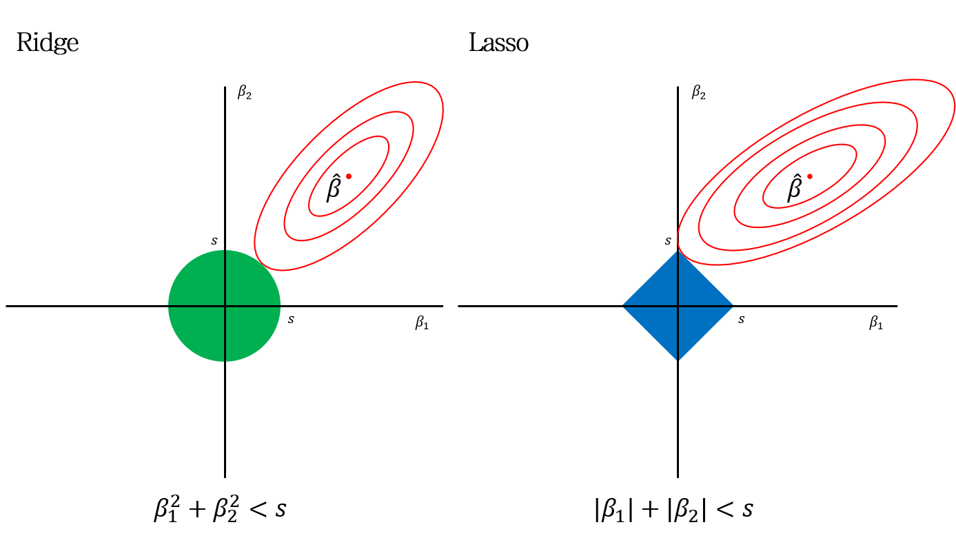
Let's analyze this visualization:

The Goal: We want to find a point within the colored constraint region that lies on the smallest possible red ellipse (i.e., has the lowest error). This point of first contact is our regularized solution.
Ridge (L2): The constraint is a circle. Because it's smooth and lacks corners, the expanding ellipse is most likely to make contact at a point where neither $β_{1}$ nor $β_{2}$ is zero. The solution is shrunk towards the origin, but it doesn't land on an axis.
Lasso (L1): The constraint is a diamond (or a hyperdiamond in higher dimensions). This shape has sharp corners that lie on the axes. As the ellipse expands, there is a high probability that it will hit one of these corners first. A point on an axis means one of the coefficients is exactly zero ( $β_{1} = 0$ or $β_{2} = 0$ ). This geometric property is the fundamental reason why Lasso performs feature selection.

Conclusion

In this lesson, we have derived L1 and L2 regularization from first principles, seeing them as solutions to constrained optimization problems. This perspective provides a solid theoretical grounding for one of the most important techniques in a machine learning practitioner's toolkit.

Here are the key takeaways:

Regularization's Goal: To prevent overfitting by adding a penalty for model complexity (large weights) to the loss function.
L2 Regularization (Ridge):
- Uses the squared L2-norm ( $∣∣ w ∣ ∣_{2}^{2}$ ) as a penalty.
- Equivalent to a constraint that the weights must lie within a hypersphere.
- It shrinks weights towards zero, an effect known as "weight decay," but rarely makes them exactly zero.
- It has a convenient closed-form solution and corresponds to a Gaussian prior on the weights.
L1 Regularization (Lasso):
- Uses the L1-norm ( $∣∣ w ∣ ∣_{1}$ ) as a penalty.
- Equivalent to a constraint that the weights must lie within a hyperdiamond.
- It can force weights to be exactly zero, thereby performing feature selection and creating sparse models.
- The objective function is non-differentiable, requiring iterative solvers like coordinate descent. It corresponds to a Laplace prior on the weights.
Geometric Intuition: The sharp corners of the L1 constraint region make it likely for the optimal solution to lie on an axis, resulting in zeroed-out weights. The smooth surface of the L2 constraint region does not share this property.

You now understand how we can intentionally modify a loss function to guide our model towards solutions that are not just accurate on the training set, but also simple and more likely to generalize.

In our next lesson, we will formalize the concept underpinning all of this: the bias-variance tradeoff. We will see that regularization is our primary tool for navigating the fundamental tension between a model that is too simple (high bias) and one that is too complex (high variance).