Polynomial Regression: Balancing Expressiveness and Overfitting

Welcome to our next lesson. In our previous discussion, we established the theoretical foundation of the bias-variance tradeoff, decomposing a model's error into its constituent parts and understanding how model complexity governs the balance between underfitting and overfitting. We saw that regularization is a tool to deliberately increase bias in order to decrease variance.

Today, we will make this abstract concept concrete. This lesson focuses on polynomial regression, a fundamental technique for introducing non-linearity into models. Our goal is to explain how polynomial regression increases a model's expressiveness and, in doing so, creates the very real risk of overfitting that we theorized about. This serves as a perfect case study for the bias-variance tradeoff in action.

From Linear to Non-Linear: The Polynomial Approach

In many real-world scenarios, the relationship between an input variable $x$ and an output $y$ is not a simple straight line. Our standard linear regression model, $y={\beta }_0+{\beta }_{1}x+ϵ$, would be a high-bias model in such cases, as it is fundamentally incapable of capturing the curvature in the data.

Polynomial regression provides a straightforward way to extend linear regression to model these non-linear relationships. We simply add higher-degree terms of the input variable to our model equation:

Here, $p$ is the degree of the polynomial. A crucial theoretical point is that while this model describes a non-linear function of $x$, it remains a linear model with respect to its coefficients ${\beta }_0,{\beta }_1,\dots ,{\beta }_p$. Because the coefficients are linear, we can still use the same ordinary least squares (OLS) machinery we developed for simple linear regression to find the optimal values for the $\beta$s.

From a data representation perspective, which should resonate with your computer science background, this is equivalent to a form of feature engineering. We create a new set of features from our original feature $x$: $x_1=x$, $x_2=x^2$, ..., $x_p=x^p$. Then, we fit a standard multiple linear regression model on these new features.

The following video provides an excellent introduction to this concept, clarifying what a polynomial is and why this method, despite its non-linear capabilities, still falls under the general linear model framework.

Expressiveness, Bias, and Variance in Action

The degree of the polynomial, $p$, is a hyperparameter that directly controls the model's complexity. As we increase $p$, we increase the model's flexibility or "expressiveness."

• A low-degree polynomial (e.g., $p=1$, a straight line) is a simple model. It will have high bias if the true underlying data relationship is curved, but its variance will be low because its shape is heavily constrained.
• A high-degree polynomial (e.g., $p=10$) is a very complex model. It can bend and curve to fit the training data very closely, leading to low bias. However, this same flexibility makes it extremely sensitive to the specific training data points, including the noise. This results in high variance.

The image below perfectly illustrates this progression. It shows nine models, from degree 1 to 9, fit to the same data. The true underlying function is the thick gray line, the training data are the blue circles, and the unseen test data are the red crosses.

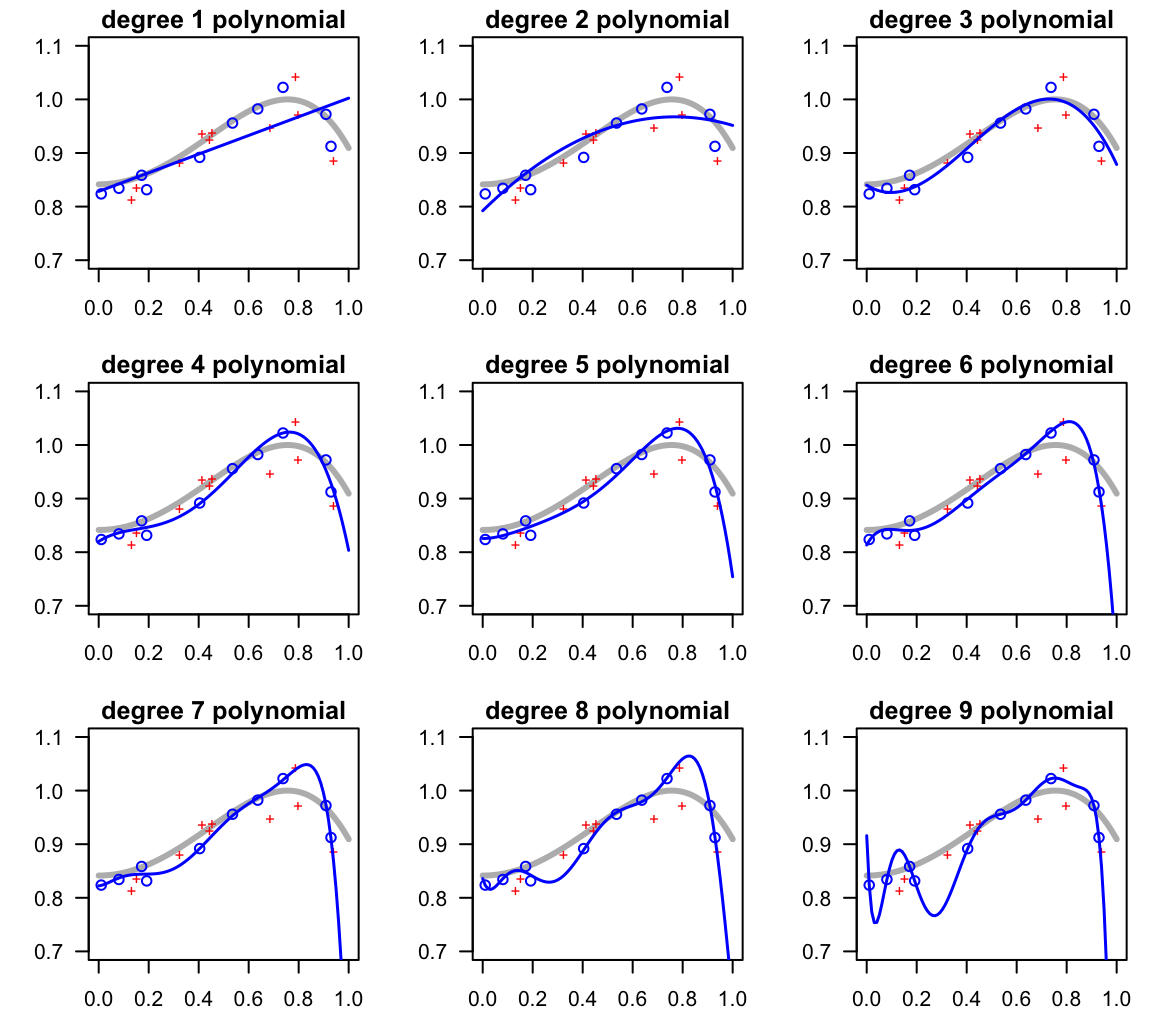
Observe the plots:

• Degree 1: Clearly underfits. It misses the overall curved trend (high bias).
• Degrees 2-4: The model begins to capture the true trend well. The fitted blue line is close to the true gray line, and it generalizes well to the red test points. This is the "sweet spot" of the bias-variance tradeoff.
• Degrees 7-9: The model starts to overfit. Notice how the blue line contorts itself to pass exactly through the training points (blue circles). This leads to wild oscillations, especially near the boundaries, causing it to miss the test points (red crosses) by a large margin. This is a classic visual of a high-variance model.

This behavior is precisely what we discussed in the last lesson. Increasing model complexity (the polynomial degree) moves us along the U-shaped curve of total error.

Choosing the Optimal Degree

The critical question is how to select the optimal degree $p$ that minimizes generalization error. As hinted at in the previous lesson and the resources above, we can't just pick the model with the lowest training error. The training error will almost always decrease as the model complexity increases.

The key is to evaluate the model on data it hasn't seen during training—a validation or test set.

The following slide deck from the University of Washington provides a clear walkthrough of this process.

The process is therefore:

1. Define a range of polynomial degrees to test (e.g., $p=1,2,\dots ,10$).
2. For each degree, train the model on the training data.
3. Evaluate the model's error (e.g., MSE) on the separate validation set.
4. Select the degree $p$ that yields the lowest validation error.
5. Optionally, retrain a final model with the chosen degree $p$ on the entire dataset (training + validation).

A Deeper Look: Why Do High-Degree Polynomials Overfit so Wildly?

The "bad reputation" of high-degree polynomials, characterized by the wild oscillations (Runge's phenomenon) seen in the plots, deserves a more rigorous explanation. Is this behavior inherent to the polynomial function class itself? A fascinating discussion on Cross Validated provides a more nuanced, expert-level answer.

The key insight is that the dramatic overfitting is not an indictment of all polynomials but a specific consequence of applying ordinary least squares to the monomial basis ($\{1,x,x^2,\dots \}$) on uniformly spaced data. Other polynomial bases (like Bernstein polynomials or Legendre polynomials) or different fitting procedures can yield high-degree polynomial models that are much more stable and less prone to overfitting. For our purposes, however, polynomial regression serves as the canonical and most intuitive example of the dangers of unchecked model complexity.

Conclusion

In this lesson, we used polynomial regression as a practical laboratory to explore the bias-variance tradeoff. We saw how increasing a model's complexity—in this case, the polynomial degree—allows it to capture more intricate patterns, thereby reducing bias. However, this same flexibility makes the model susceptible to fitting noise, which increases variance and leads to overfitting.

Key Takeaways:

• Polynomial Regression extends linear models by adding higher-power terms of the input variables, enabling it to fit non-linear data.
• It is still a linear model in its coefficients and can be solved with ordinary least squares.
• The polynomial degree is a hyperparameter that controls model complexity.
• Increasing the degree reduces bias but increases variance. This creates a direct and observable bias-variance tradeoff.
• The optimal degree is found not by minimizing training error, but by finding the model that performs best on a separate validation set, typically at the bottom of a U-shaped test error curve.
• The extreme instability of high-degree polynomial fits is a result of the standard fitting procedure on the monomial basis, which mathematically leads to an exponential growth in variance.

We have now seen why it is crucial to evaluate a model on data it has not been trained on. In our next lesson, we will formalize this practice by examining the train/validation/test split methodology, a cornerstone of reliable and unbiased machine learning practice.