Roofline Model: Arithmetic Intensity & Memory Bandwidth

Introduction

In our last two lessons, we mapped out the GPU's memory hierarchy and investigated memory coalescing, the key to achieving high effective bandwidth from slow global memory. We established that how you access data is just as important as how much data you need. But this raises a crucial question: when you're optimizing a kernel, should you focus on reducing memory traffic, or is the bottleneck somewhere else?

This lesson introduces a powerful tool for answering that question: the Roofline model. It's an intuitive, visual model that connects a processor's peak performance and memory bandwidth to the characteristics of your specific algorithm. By using it, you can determine whether your program is limited by computation or by memory access, which in turn tells you exactly where to focus your optimization efforts.

This directly supports your goal of understanding how to design and optimize systems for AI, as the Roofline model is a standard tool for analyzing the performance of deep learning workloads.

Our learning outcome for today is to: Analyze the relationship between arithmetic intensity and memory bandwidth using the Roofline model.

By the end of this lesson, you will be able to:

• Define the core components of the Roofline model: peak performance, peak bandwidth, and arithmetic intensity.
• Construct and interpret a Roofline plot for a given hardware configuration.
• Calculate the arithmetic intensity of a simple kernel.
• Use the model to diagnose whether a kernel is compute-bound or memory-bound and identify promising optimization strategies.

1. The Core Concepts of the Roofline Model

At its heart, the Roofline model simplifies a complex computer system into two fundamental performance limits and characterizes a program with a single metric.

1. Hardware Ceilings:

   • Peak Performance ($P_{\text{peak}}$): The maximum rate of computation the processor can sustain, typically measured in Floating Point Operations Per Second (FLOP/s). This is the compute roof.
   • Peak Memory Bandwidth ($B_{\text{peak}}$): The maximum rate at which data can be moved between the processor and main memory, measured in Bytes per Second (B/s). This is the memory roof.

2. Software Characterization:

   • Arithmetic Intensity ($I$): The ratio of floating-point operations performed to the total bytes of data moved to and from main memory for a given kernel. The unit is FLOP/Byte.

A kernel with high arithmetic intensity performs many calculations for each byte it reads, while one with low intensity is "chatty," requiring a lot of data for relatively few computations.

To see how these components come together, please watch the following video, which provides a clear and concise introduction to the model's derivation.

As the video explained, the attainable performance $P$ of any kernel is capped by the minimum of two values: its potential performance if limited only by computation, and its potential performance if limited only by memory bandwidth.

This gives us the fundamental Roofline equation:

Graphically, this creates the characteristic "roofline" shape: a sloped line representing the memory bandwidth limit, and a flat horizontal line representing the peak compute limit.

2. A Practical GPU Example

Let's make this concrete by applying the model to a modern GPU. The concepts are theoretical, but their application requires real hardware specifications.

We'll use the NVIDIA A100 GPU as our example. Please read the following text, which provides its key performance numbers and uses them to build a Roofline model. It then analyzes a simple matrix multiplication kernel.

Let's summarize the key calculations from the resource:

• Hardware (A100):
  • $P_{\text{peak}}$ = 19,500 GFLOP/s (for FP32)
  • $B_{\text{peak}}$ = 1,555 GB/s
• The "Ridge Point" ($I^{\ast }$): This is the point where the memory roof meets the compute roof. It represents the minimum arithmetic intensity a kernel needs to have a chance of becoming compute-bound. $$I^{\ast }=\frac{P_{\text{peak}}}{B_{\text{peak}}}=\frac{19,500\text{ GFLOP/s}}{1,555\text{ GB/s}}\approx 12.5\text{ FLOP/Byte}$$
• Software (Naive MatMul):
  • For each output element, the kernel performs $2N-1$ FLOPs and reads $2N$ matrix elements from global memory. For $N=2$, this is 3 FLOPs and 16 bytes.
  • $I_{\text{naive}}=\frac{3\text{ FLOPs}}{16\text{ Bytes}}=0.1875\text{ FLOP/Byte}$
• Analysis:
  Since $I_{\text{naive}}\ll I^{\ast }$, the kernel is severely memory-bound. Its performance is limited by the sloped part of the roof. The theoretical peak performance for this specific kernel is: $$P_{\text{naive}}=I_{\text{naive}}\times B_{\text{peak}}=0.1875\times 1,555\approx 292\text{ GFLOP/s}$$ This is only about 1.5% of the A100's peak computational capability! The GPU is spending most of its time waiting for data.

3. The Roofline as an Optimization Compass

The true power of the Roofline model is its ability to guide optimization. By plotting where your kernel lies, it tells you what kind of optimization will be most effective.

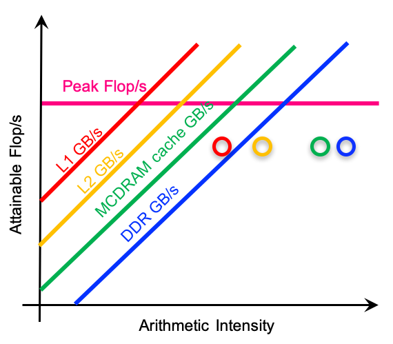
If your kernel is memory-bound ($I<I^{\ast }$):
Your goal is to move its data point up and to the right on the plot.

1. Move Up (Increase Effective Bandwidth): For a given arithmetic intensity, performance is $P=I\times B$. To increase $P$, you must increase $B$. This is where the lesson on memory coalescing becomes critical. By improving your access patterns, you raise your effective memory bandwidth closer to the hardware's peak, moving your kernel's performance vertically towards the memory roof.
2. Move Right (Increase Arithmetic Intensity): To cross the ridge point and become compute-bound, you must increase the FLOP-to-byte ratio. This involves algorithmic changes to reduce memory traffic. Common techniques include:
   • Data Reuse: Use fast on-chip memory (like shared memory or registers) to load data once and use it many times. This is the core idea behind tiled matrix multiplication.
   • Operator Fusion: Combine multiple consecutive kernels (e.g., a convolution followed by a ReLU activation) into a single kernel. This eliminates the need to write the intermediate result to global memory and immediately read it back, effectively increasing the number of FLOPs performed per byte loaded from DRAM.

The following figure from a recent research paper on LLM inference clearly illustrates the effect of operator fusion.

If your kernel is compute-bound ($I>I^{\ast }$):
Your kernel is already performing enough work per byte to saturate the compute units. Improving memory access patterns won't yield significant gains. Instead, you should focus on:

• Instruction-Level Parallelism: Ensure the compiler is generating efficient machine code.
• Using more powerful ALUs: For example, moving from 32-bit floating-point (FP32) math to 16-bit (FP16/BF16) or using specialized units like Tensor Cores can dramatically increase $P_{\text{peak}}$.

4. Application to Real-World ML Workloads

The Roofline model is not just an academic exercise; it is a vital tool for engineers designing and optimizing the systems that run large-scale AI. Given your background and goals, seeing its direct application to a state-of-the-art model is crucial.

The same paper on LLM inference provides a fascinating table where they perform a Roofline analysis for each layer of the Llama-2-7B model.

This analysis is incredibly revealing. It shows that even within a single model, the performance bottleneck can change dramatically depending on the workload (e.g., prefill vs. decode). This is a prime example of how systems-level thinking and performance analysis are essential for building efficient AI infrastructure.

Conclusion

In this lesson, we demystified the relationship between computation and memory bandwidth using the Roofline model. It provides a robust, quantitative framework for performance analysis that moves beyond guesswork and pinpoints the true limiting factor for your code.

Key Takeaways:

• The performance of a GPU kernel is bound by the minimum of its compute ceiling ($P_{\text{peak}}$) and its memory ceiling ($I\times B_{\text{peak}}$).
• Arithmetic Intensity ($I$) is the key property of an algorithm that determines which ceiling is the limiter.
• The Ridge Point ($I^{\ast }=P_{\text{peak}}/B_{\text{peak}}$) separates memory-bound kernels from compute-bound kernels.
• The Roofline model is a powerful diagnostic tool and an optimization guide:
  • For memory-bound kernels, focus on improving effective bandwidth (e.g., coalescing) or increasing arithmetic intensity (e.g., data reuse, kernel fusion).
  • For compute-bound kernels, focus on using more efficient computations (e.g., reduced precision).

Preview of the Next Lesson:

We've now built a solid conceptual tool for analyzing performance. As we saw in the Llama-2-7B example, many critical ML workloads are, in fact, memory-bound. In the next lesson, "Explain how memory bandwidth can become a bottleneck in data-intensive ML workloads," we will delve deeper into why this is the case. We will examine the operational characteristics of common ML layers, like attention and large linear layers, to understand why their arithmetic intensity is often low, making memory bandwidth a primary constraint on end-to-end performance.