Memory Bandwidth Bottlenecks in Data-Intensive ML

Introduction

Welcome back. In our previous lesson, we introduced the Roofline model as a powerful tool for analyzing kernel performance. We established that a program's performance is limited by either its computational throughput or its memory bandwidth, and that the key determinant is its arithmetic intensity—the ratio of computations to data movement. We even saw a preview of today's topic when we noted that the "decode" phase of a large language model is often memory-bound.

Today, we will explore this phenomenon in depth. Your goal is to understand how to design and optimize AI systems, and a critical part of that is recognizing the primary performance limiters. For many of the most important modern AI workloads, that limiter is memory bandwidth. This lesson will explain exactly why that is the case.

Our learning outcome is to: Explain how memory bandwidth can become a bottleneck in data-intensive ML workloads.

We will cover:

• The concept of the "memory wall" and the growing disparity between compute power and memory bandwidth.
• A detailed case study of Transformer inference, dissecting why processing a prompt (prefill) and generating a response (decode) have fundamentally different performance characteristics.
• The role of the growing KV cache in exacerbating memory pressure during inference.
• How these factors lead to underutilization of expensive compute hardware, directly impacting system performance and cost.

1. The "Memory Wall": A Widening Chasm

The idea that memory access is a bottleneck is not new. It's a long-standing challenge in computer architecture known as the memory wall. This term describes the growing gap between the rate at which processors can perform computations and the rate at which they can be supplied with data from memory.

As you know from your background, processor performance (driven by transistor density and clock speed, as described by Moore's Law) has historically scaled at a much faster exponential rate than memory bandwidth. For AI accelerators like GPUs, this trend is even more pronounced. They pack immense computational power (measured in TFLOP/s), but the improvements in memory and interconnect bandwidth lag significantly behind.

Let's look at some data that illustrates this trend.

The key takeaway from this reading is the stark difference in scaling exponents. While peak compute has skyrocketed (a 60,000x increase in 20 years!), DRAM bandwidth has only increased by about 100x. This disparity means that for an application to effectively use all that computational power, it must perform a very large number of operations for every byte of data it fetches from memory. In other words, it must have a very high arithmetic intensity.

As we are about to see, many crucial ML workloads do not.

2. A Tale of Two Workloads: Prefill vs. Decode

Nowhere is the memory bandwidth bottleneck more apparent than in the inference of autoregressive models like Transformers (the architecture behind models like GPT-4). While we often talk about "inference" as a single process, it's actually comprised of two distinct phases with radically different performance profiles: prefill and decode.

The following article provides one of the clearest explanations available of this dichotomy and its relationship to hardware performance. We will use it as the backbone for the rest of this lesson.

Let's consolidate the crucial insights from that reading.

2.1. Prefill: A Compute-Bound Task

• What it is: The initial processing of the user's input prompt.
• How it works: All tokens in the prompt are known, so they can be processed in parallel. The core operations are large matrix-matrix multiplications (e.g., input sequence matrix X of size [n, d] multiplied by weight matrix W of size [d, d]).
• Arithmetic Intensity: As calculated in the article, the intensity is approximately $I_{\text{prefill}}\approx 2n/B_p$, where n is the sequence length and B_p is bytes per parameter.
  • For a prompt of n=4096 tokens and FP16 precision (B_p=2), the arithmetic intensity is ~4096 FLOPs/byte.
• Roofline Analysis: This intensity is far greater than the ridge point of a modern GPU like the H100 (~295 FLOPs/byte). This places the prefill phase squarely in the compute-bound regime. The GPU's performance is limited by its raw TFLOP/s, and its massive parallelism is well-utilized.

2.2. Decode: A Memory-Bound Bottleneck

• What it is: The step-by-step generation of the output sequence.
• How it works: Output is generated one token at a time, as each new token depends on the previous one. This is an inherently serial, or autoregressive, process. The core operations become matrix-vector multiplications (e.g., a single new token's vector of size [1, d] multiplied by the weight matrices of size [d, d]).
• Arithmetic Intensity: The intensity collapses to $I_{\text{decode}}\approx 2/B_p$.
  • For FP16 (B_p=2), this is just 1 FLOP/byte.
• Roofline Analysis: An intensity of 1 is far, far below the GPU's ridge point. This places the decode phase deep in the memory-bound regime. Performance is now dictated by the memory ceiling: $P_{\text{decode}}=I_{\text{decode}}\times B_{\text{peak}}$.
  • With an H100's bandwidth of ~3350 GB/s, the attainable performance is a mere 3.35 TFLOP/s, which is less than 1% of the chip's FP16 compute capability (~989 TFLOP/s).

This is the essence of the memory bottleneck in data-intensive ML. During the token generation phase—the part that determines the user-perceived speed (tokens-per-second)—the most powerful AI accelerators in the world are almost entirely idle, waiting for data to be shuttled from memory.

3. The Compounding Factor: The KV Cache

The situation during the decode phase is actually even more constrained than just loading model weights. The attention mechanism requires that each new token "looks at" all previous tokens in the sequence. To avoid ruinously expensive recomputation, the intermediate Key (K) and Value (V) vectors for each token are stored in a KV cache.

This cache has a direct and significant impact on the memory bottleneck.

As the article highlights, the total data moved during a single decode step is not just the model weights; it's the model weights + the current KV cache.

• Model Weights: A fixed size per step (e.g., ~7GB for a 14B model at INT4).
• KV Cache: Grows linearly with every token generated. For a long context, the cache can become several gigabytes in size, sometimes even larger than the model weights themselves.

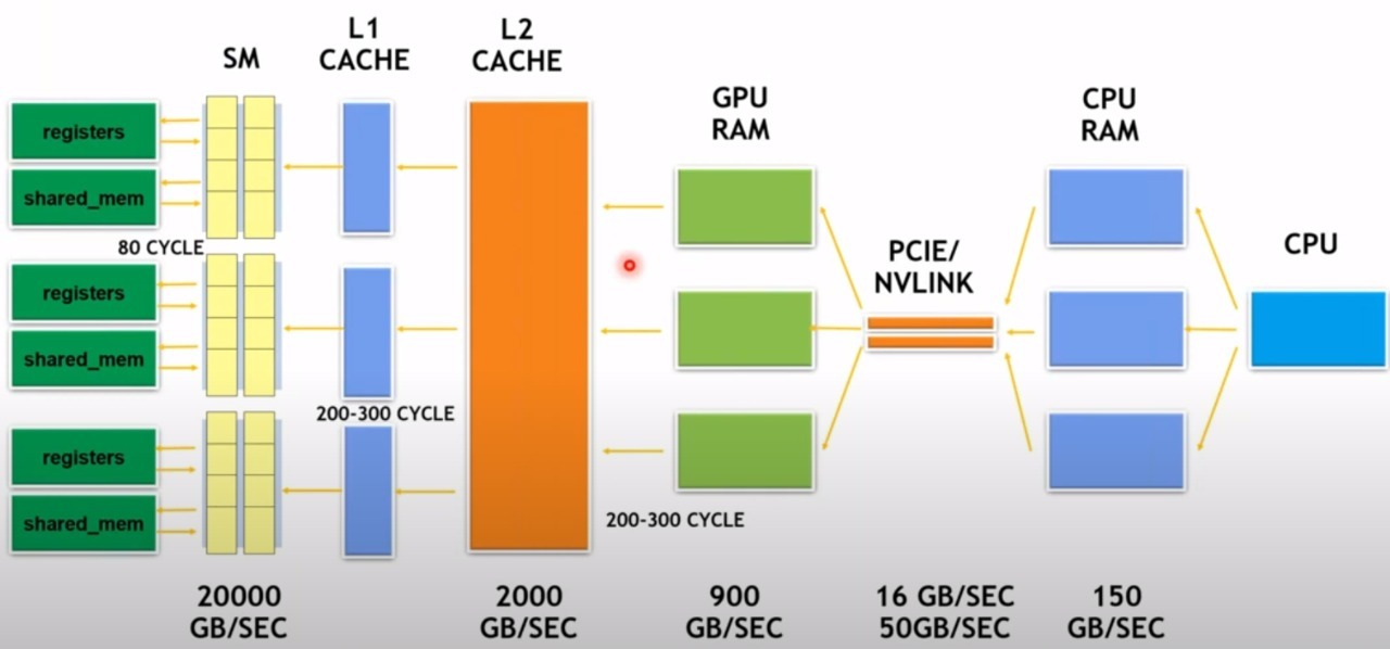
This means that as the output sequence gets longer, each generation step becomes slower because more and more data (the growing cache) must be read from the slow main GPU memory (DRAM/HBM), further stressing the memory bandwidth.

Let's visualize where this bottleneck sits within the GPU's memory hierarchy.

Conclusion

In this lesson, we moved from the abstract concept of a memory-bound workload to a concrete, quantitative understanding of why this is the reality for many data-intensive AI models.

Key Takeaways:

• The memory wall is the growing divergence between compute performance and memory bandwidth, making memory access a primary bottleneck for modern systems.
• Transformer inference is a prime example, consisting of two distinct phases:
  • Prefill (compute-bound): Parallel, high-intensity matrix-matrix operations that efficiently use the GPU's compute units.
  • Decode (memory-bound): Autoregressive, low-intensity matrix-vector operations where performance is limited by memory bandwidth, leaving compute units mostly idle.
• The KV cache, necessary for efficient attention, grows with the context length. During decode, reading this growing cache from DRAM adds to the memory pressure, making each successive token generation step slower.
• Ultimately, for a memory-bound workload, performance is a direct function of memory bandwidth. Doubling a chip's TFLOP/s will yield almost no improvement; you must increase the bytes per second it can move from its main memory.

Preview of the Next Lesson:

We've firmly established that memory bandwidth is a critical resource. This naturally leads to the question: what technologies are used to provide this bandwidth, and what are their trade-offs? In the next lesson, we will compare the two dominant memory technologies used in GPUs—High Bandwidth Memory (HBM) and GDDR—analyzing their differences in performance, power consumption, and cost. This will complete our foundational understanding of the GPU memory system, from its hierarchical structure to the physical technologies that underpin it.