Memory Coalescing and Bandwidth Optimization

Introduction

Welcome back! In our previous lesson, we constructed a map of the GPU's memory hierarchy. We learned that while off-chip global memory (DRAM) is vast, it's also the slowest tier, with access latencies hundreds of times higher than on-chip registers. The GPU's primary strategy to overcome this is to fetch data in massive, parallel chunks to achieve high peak bandwidth.

However, this peak bandwidth is a theoretical maximum. The actual data rate you achieve—the effective bandwidth—is critically dependent on how you access that memory. This lesson is dedicated to the single most important principle for optimizing global memory performance.

We will focus on the learning outcome: Explain the concept of memory coalescing and its impact on effective bandwidth.

By the end of this lesson, you will understand:

• The link between the GPU's parallel execution model (warps) and the physical organization of DRAM.
• How memory access patterns of threads within a warp determine the number of physical memory transactions.
• The definition of memory coalescing and why it is the key to unlocking high effective bandwidth.

1. From Logical Accesses to Physical Transactions

Let's start with a practical demonstration. Imagine two different ways to write a matrix multiplication kernel. One maps threads to rows, the other maps them to columns. Logically, both are correct, yet one can be over 4 times faster. Why? The answer lies in the interaction between the GPU's execution model and the memory hardware.

As the video explains, the core principle is this:

1. DRAM works in bursts: To amortize the high latency of accessing a memory location, DRAM controllers are designed to fetch not just a single byte, but a whole block of contiguous data (a "burst" or "cache line") in one operation.
2. Warps access memory together: All 32 threads in a warp execute the same instruction in lockstep. When this instruction is a load from global memory, the hardware attempts to service all 32 memory requests simultaneously.

This leads us to the central idea: if the memory addresses requested by the 32 threads in a warp are contiguous and aligned, the memory controller can satisfy all of them with a single, efficient DRAM burst. This is memory coalescing.

The hardware combines, or coalesces, multiple logical memory requests into a single physical transaction.

Conversely, if the threads request data from scattered, non-contiguous memory locations, the hardware has no choice but to issue multiple, separate transactions. This serialization of requests destroys the parallelism of the memory system, causing the effective bandwidth to plummet.

Let's read a formal definition to solidify this concept.

2. The Key: Access Patterns and Data Layout

So, how do we ensure threads in a warp access consecutive memory locations? This depends entirely on two factors you control as a programmer:

1. How you map threads to data.
2. How that data is laid out in linear memory.

Your background in computer science is directly applicable here. You know that multi-dimensional data structures, like matrices, must be flattened into a one-dimensional address space. Most C-like languages and frameworks like PyTorch use row-major order, where elements of a row are contiguous in memory.

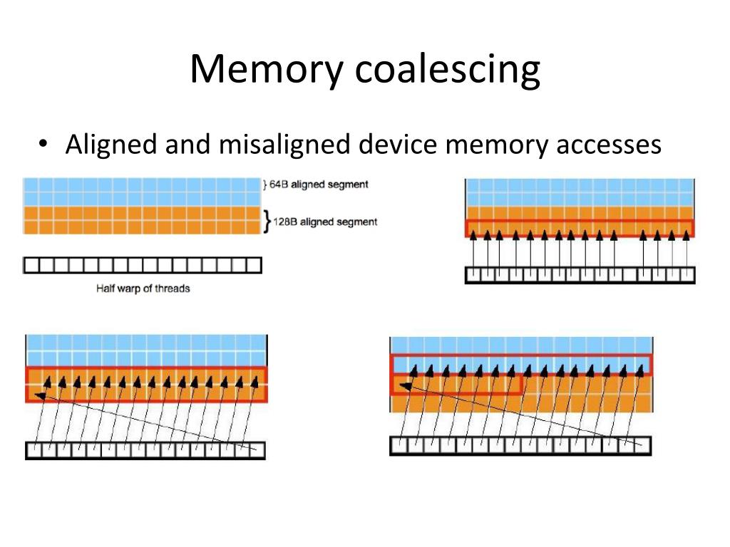
Let's consider accessing a 2D matrix M in a row-major layout:

• Coalesced Access (Good): Imagine threads in a warp process a row of M. Thread 0 accesses M[i][j], thread 1 accesses M[i][j+1], thread 2 accesses M[i][j+2], and so on. Since these elements are adjacent in memory, this access pattern is perfectly coalesced.

• Non-Coalesced Access (Bad): Now, imagine the threads process a column. Thread 0 accesses M[i][j], thread 1 accesses M[i+1][j], thread 2 accesses M[i+2][j], etc. In a row-major layout, these elements are far apart in memory, separated by the stride of the matrix (i.e., the length of a full row). This is a strided access pattern and it is not coalesced.

The following video provides a great walkthrough of this exact scenario in the context of matrix multiplication.

This principle—aligning your thread access patterns with the underlying data layout—is the most fundamental optimization for any memory-bound GPU kernel. An algorithm that looks elegant on paper can perform terribly if it results in scattered memory accesses. This is why you often see data preprocessing steps in high-performance code, such as transposing a matrix, purely to ensure that subsequent kernel launches can use coalesced memory patterns.

3. Quantifying the Impact on Effective Bandwidth

We can be more precise about the performance penalty of non-coalesced access. A warp-level memory instruction can generate anywhere from 1 to 32 physical transactions to global memory.

• Best Case: A perfectly coalesced load of 32 four-byte floats (128 bytes total) can be serviced by a single 128-byte memory transaction.
• Worst Case: A "gather" operation, where each of the 32 threads accesses a random, unrelated address, could require 32 separate 32-byte transactions (assuming a 32-byte cache line granularity). This is because each access falls into a different memory segment.

The effective bandwidth is directly proportional to the number of bytes transferred and inversely proportional to the number of transactions required.

$\text{Effective Bandwidth}=\frac{\text{Total Bytes Transferred}}{\text{Time Taken}}$

Since each transaction has a fixed latency overhead, issuing 32 transactions takes much longer than issuing one, even if the total amount of data is similar. This drastically increases the "Time Taken" and crushes the effective bandwidth.

The academic paper "An Instruction Roofline Model for GPUs" (which we will revisit later in the course) offers a precise way to think about this. It characterizes memory access patterns by their "Instruction Intensity," defined as warp-level instructions per transaction.

Let's look at their case study of a matrix transpose operation, which is all about memory movement.

The paper's experiment is a perfect summary:

1. Naive Transpose: Reads a column from the input matrix (coalesced) and writes to a column in the output matrix. Since the output matrix is stored row-major, writing to a column is a highly strided, non-coalesced operation. The paper notes this results in the worst-case scenario: 32 separate transactions per warp.
2. Optimized Transpose: Uses on-chip shared memory as a staging area. It performs a coalesced read from global memory into shared memory, performs the transpose entirely within fast shared memory, and then performs a coalesced write from shared memory back to global memory.

This demonstrates a critical design pattern in GPU computing: use fast, on-chip shared memory to rearrange data to enable coalesced access to slow, off-chip global memory.

Conclusion

In this lesson, we dissected the concept of memory coalescing and established its paramount importance for GPU performance. By aligning your application's memory access patterns with the hardware's capabilities, you can transform a memory-bound bottleneck into a highly efficient data pipeline.

Key Takeaways:

• Memory Coalescing: A hardware feature that merges memory requests from threads in a warp into a small number of physical memory transactions.
• The Condition: Coalescing occurs when consecutive threads access consecutive memory locations. This requires awareness of the underlying data layout (e.g., row-major order).
• The Impact: Coalesced access maximizes effective memory bandwidth by minimizing the number of slow physical transactions.
• Non-Coalesced Access: Strided or random access patterns force the hardware to issue many separate transactions, severely degrading effective bandwidth and stalling the GPU's computational units.
• Optimization Strategy: A common and powerful pattern is to load data into on-chip shared memory using coalesced reads, rearrange it, and then write it back to global memory using coalesced writes.

It's worth noting that a similar principle, called bank conflicts, applies to on-chip shared memory. Accesses to shared memory can also be serialized if multiple threads in a warp try to access different addresses that fall into the same memory bank. This reinforces the core idea that access patterns matter at every level of the memory hierarchy.

Preview of the Next Lesson:

We now understand the components of the memory hierarchy (Lesson 2.1) and the primary mechanism for using it efficiently (this lesson). We are now equipped to analyze the performance of a kernel as a whole. In the next lesson, we will revisit the Roofline model, which provides a formal framework for analyzing whether a given algorithm is limited by the GPU's computational power or its memory bandwidth. Your understanding of effective bandwidth will be crucial for interpreting this model correctly.