Representing 3D Scenes with Anisotropic Gaussian Primitives

In our previous module, we concluded our deep dive into Neural Radiance Fields. You deconstructed the original paper, understanding NeRF as a powerful, implicit representation of a scene. However, we also identified its primary weakness, one that is especially relevant to your interests in performance systems: NeRF is slow. Rendering a single image requires millions of queries to a neural network, a process that is far from real-time.

This lesson marks our transition to a technique designed specifically to overcome this limitation: 3D Gaussian Splatting (3DGS). We will explore a fundamental shift in philosophy, moving away from NeRF's implicit function towards an explicit, geometric representation. Your goal for this lesson is to understand precisely what these new geometric primitives are and how they combine to represent a photorealistic 3D scene.

From Implicit Functions to Explicit Primitives

Let's begin by solidifying the distinction between the two approaches. NeRF represents a scene as a continuous, implicit function $F_{\Theta }$ stored in the weights of an MLP. To find the color and density at any point $\mathbf{x}$, you must execute a forward pass through the network: $(\mathbf{c},\sigma )=F_{\Theta }(\mathbf{x},\mathbf{d})$. The scene is the function.

3D Gaussian Splatting rejects this paradigm. From a systems perspective, repeatedly querying a large function is inefficient. A more direct approach, common in traditional computer graphics, is to represent a scene as a list of discrete objects, or primitives (e.g., a mesh is a list of triangles). 3DGS adopts this explicit philosophy but chooses a different, more flexible primitive: the 3D Gaussian.

To get a high-level overview of this shift, let's watch a segment from a lecture that introduces 3DGS and contrasts it directly with NeRF.

As the video explains, instead of a single, complex function, a 3DGS scene is a collection of millions of simpler, localized objects. The core task now is to understand the properties of these objects.

The Primitive: Anisotropic 3D Gaussians

The fundamental building block of a 3DGS scene is the 3D Gaussian. Imagine filling a 3D space with millions of semi-transparent, colored ellipsoids to "sculpt" the scene. Where NeRF learns a function, 3DGS learns the optimal position, shape, color, and transparency of each of these ellipsoids.

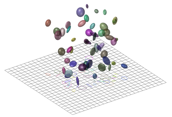
So, what defines one of these primitives? Each 3D Gaussian is characterized by a set of optimizable parameters. Let's examine each one.

As you just saw, each Gaussian primitive is defined by the following properties:

1. Position (Mean $\mu$): A 3D vector $\mathbf{x}=(x,y,z)$ that specifies the center of the Gaussian. This is analogous to the mean of a Gaussian distribution.

2. Covariance ($\Sigma$): A 3x3 matrix that defines the Gaussian's shape. This is the key to the anisotropy of the primitive. While a single number (variance) defines the width of a 1D Gaussian, a covariance matrix defines the shape and orientation of a 3D Gaussian, allowing it to be an ellipsoid rather than just a sphere.

3. Opacity ($\alpha$): A scalar value that controls the transparency of the Gaussian. This is analogous to the density $\sigma$ in NeRF and is crucial for rendering complex geometry and semi-transparent objects.

4. Color (via Spherical Harmonics): To handle view-dependent effects (like shininess), the color is not a single RGB value. Instead, each Gaussian stores a set of Spherical Harmonic (SH) coefficients. We will explore these in more detail shortly.

This set of parameters—position, covariance, opacity, and color coefficients—forms the complete description of a single primitive. The entire scene is simply a large list containing millions of these parameter sets.

Anisotropy and the Covariance Matrix

The term anisotropic is critical. It means "directionally dependent." An isotropic primitive would be a sphere, having the same size in all directions. An anisotropic primitive, our ellipsoid, can be stretched, squashed, and rotated to more efficiently represent flat surfaces or elongated structures. A single large, flat ellipsoid can cover a piece of a wall, whereas it would take thousands of tiny spheres to do the same job. This efficiency is enabled entirely by the covariance matrix $\Sigma$.

From our study of linear algebra, you'll recall the geometric interpretation of eigendecomposition. The same principle applies here:

• The eigenvectors of the covariance matrix $\Sigma$ determine the orientation of the ellipsoid's principal axes (its rotation in 3D space).
• The eigenvalues of $\Sigma$ determine the length of these axes (its scale).

Now, consider the optimization process. We need to find the optimal $\Sigma$ for each Gaussian using gradient descent. However, a covariance matrix must always be positive semi-definite (PSD). A standard gradient update on the nine elements of the matrix does not guarantee this property, and an invalid matrix could break the physics of the model.

Question: How might you ensure a matrix remains positive semi-definite throughout an optimization process? Think about matrix decompositions. Is there a way to construct the matrix from components that are easier to optimize without constraints?

The authors of 3DGS solve this with an elegant engineering choice. Instead of optimizing $\Sigma$ directly, they optimize two simpler components:

• A 3D scale vector $\mathbf{s}$
• A 4D rotation vector $\mathbf{q}$ (a quaternion)

These are then used to form a rotation matrix $\mathbf{R}$ (from $\mathbf{q}$) and a scaling matrix $\mathbf{S}$ (from $\mathbf{s}$). The final covariance matrix is constructed as:

This construction mathematically guarantees that the resulting $\Sigma$ will always be positive semi-definite, allowing for stable and unconstrained optimization of scale and rotation.

The following reading explains this decomposition clearly.

Color and View-Dependence with Spherical Harmonics

Just as in NeRF, we need to model how the appearance of a surface can change depending on the viewing angle. NeRF accomplished this by feeding the viewing direction vector $\mathbf{d}$ into its MLP. 3DGS uses a different mechanism rooted in classical graphics: Spherical Harmonics (SH).

Think of SH as the 3D equivalent of a Fourier series. A Fourier series can represent a complex 1D signal as a weighted sum of simple sine and cosine basis functions. Similarly, spherical harmonics are a set of basis functions defined on the surface of a sphere. Any function on a sphere—such as "the color of an object as viewed from any direction"—can be approximated as a weighted sum of these SH basis functions.

Instead of storing a static RGB value, each Gaussian stores the coefficients for this weighted sum. During rendering, the viewing direction is used to evaluate this SH function, producing the correct view-dependent color.

Conclusion

In this lesson, we have transitioned from NeRF's implicit world to the explicit, object-centric representation of 3D Gaussian Splatting. You have seen that this choice is fundamentally motivated by the pursuit of performance, a theme that resonates with your background in systems engineering.

Key Takeaways:

• Explicit Representation: A 3DGS scene is represented by a collection of millions of explicit primitives, not by a neural network.
• Anisotropic Primitives: The chosen primitive is the 3D Gaussian, which is visualized as an ellipsoid. Its anisotropic nature (ability to be scaled and rotated non-uniformly) allows it to represent scene geometry much more efficiently than isotropic primitives like spheres.
• Gaussian Parameters: Each primitive is defined by a set of optimizable parameters:
  • Position: The 3D mean $\mu$.
  • Covariance: A 3x3 PSD matrix $\Sigma$, which is stored and optimized as separate scale ($\mathbf{s}$) and rotation ($\mathbf{q}$) components to ensure validity.
  • Opacity: A scalar $\alpha$ controlling transparency.
  • Color: A set of Spherical Harmonic coefficients to model view-dependent effects.

Preview of the Next Lesson:

We now understand what a 3DGS scene is made of. The next logical question is: how do we create a 2D image from this 3D collection of Gaussians? In the next lesson, we will investigate the rendering pipeline. We'll cover the mathematics of projecting a 3D Gaussian ellipsoid onto a 2D image plane to become an elliptical "splat" and begin to explore the highly optimized, differentiable rasterization process that enables 3DGS to achieve its remarkable real-time rendering speeds.