Price Elasticity of Supply

Hello! Welcome to our next lesson in the "Supply, Demand, and Market Equilibrium" module.

In our last few lessons, we've focused entirely on the demand side of the market. We explored price elasticity of demand (PED), which measures how consumers' buying habits respond to price changes, and then delved into cross-price and income elasticities to understand how other factors influence demand.

Now, it's time to switch our perspective to the producers. Just as we measured consumer sensitivity, we also need a tool to measure producer sensitivity to price changes. This is where the Price Elasticity of Supply (PES) comes in.

Our learning outcome for this lesson is to explain price elasticity of supply and its determinants. By the end of this session, you will be able to:

• Define and calculate the price elasticity of supply.
• Interpret its value to determine if supply is elastic or inelastic.
• Identify and explain the key factors that make the supply of a good more or less responsive to price changes.

This concept is crucial for understanding why some markets can adapt quickly to new conditions while others respond much more slowly.

1. Defining Price Elasticity of Supply

Price Elasticity of Supply (PES) measures how much the quantity supplied of a good responds to a change in its price. In simple terms, it tells us how willing and able firms are to increase production when the price of their product goes up.

The formula is very similar to the one for price elasticity of demand:

$$\text{PES}=\frac{\text{\% Change in Quantity Supplied}}{\text{\% Change in Price}}$$

A key difference from PED is that PES will almost always be a positive number. This is due to the Law of Supply: a higher price gives producers an incentive to supply more, so price and quantity supplied move in the same direction. Therefore, we don't need to drop any negative signs; we interpret the positive value directly.

To get a quick and clear introduction to the concept and its calculation, please watch the first part of the following video.

2. Interpreting the Values of PES

As the video explained, the magnitude of the PES value tells us how responsive producers are. We can categorize supply into five types based on this value.

The following reading from your textbook, Economics for the IB Diploma, provides a formal breakdown of these categories and their graphical representations.

Here is a summary of the key classifications:

• Inelastic Supply (0 < PES < 1): The percentage change in quantity supplied is smaller than the percentage change in price. Producers are not very responsive to price changes. The supply curve is steep.
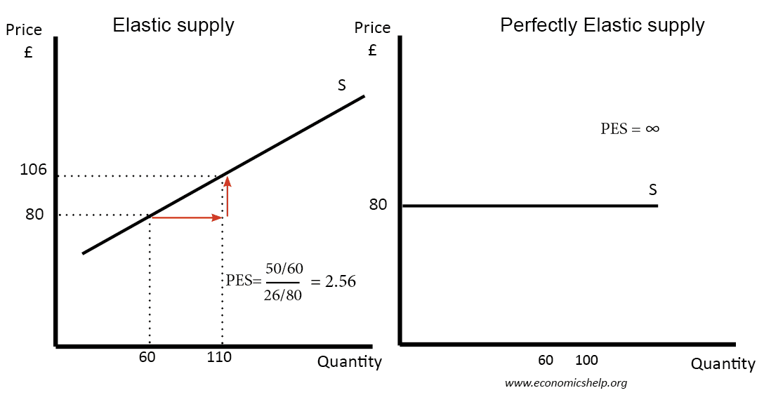
• Elastic Supply (PES > 1): The percentage change in quantity supplied is larger than the percentage change in price. Producers are very responsive to price changes. The supply curve is relatively flat.
• Unit Elastic Supply (PES = 1): The percentage change in quantity supplied is exactly equal to the percentage change in price. Any straight-line supply curve that passes through the origin (0,0) is unit elastic.
• Perfectly Inelastic Supply (PES = 0): The quantity supplied does not change at all, regardless of the price. The supply curve is a vertical line. Think of the supply of unique items like the Mona Lisa or the number of seats in a stadium.
• Perfectly Elastic Supply (PES = ∞): Producers are willing to supply any amount at a specific price, but nothing at a lower price. The supply curve is a horizontal line.

3. The Determinants of Price Elasticity of Supply

Now for the most important part of our lesson: what makes supply elastic or inelastic? A firm's ability to respond to a price change isn't a matter of choice; it's constrained by several practical factors.

The following video from Marginal Revolution University offers an excellent, intuitive explanation of these determinants with clear, memorable examples.

Let's summarize the key determinants discussed in the video and our other resources:

1. Time Horizon: This is arguably the most critical factor.

   • Short Run: Supply is typically inelastic because firms have at least one fixed factor of production (like the size of their factory). They can't easily change their output.
   • Long Run: Supply becomes more elastic because all factors of production are variable. Firms can build new factories, purchase more machinery, or train more workers, allowing for a much larger response to a sustained price change.

2. Availability of Inputs & Factor Mobility: If a firm can easily acquire the necessary raw materials, labor, and capital, it can increase production quickly, making supply more elastic. If key inputs are scarce or it's hard to shift resources from making other products, supply will be more inelastic.

3. Spare Production Capacity: If a firm has unused machinery or idle workers, it can respond to a price increase almost instantly by putting these resources to work. The more spare capacity a firm or industry has, the more elastic its supply.

4. Ability to Store Stocks (Inventories): For goods that are not perishable, firms can hold inventories. If the price rises, they can sell these stocks, leading to a highly elastic supply in the very short term. Once inventories are depleted, elasticity depends on production capacity.

5. Complexity and Length of Production: Goods that are simple and quick to produce (e.g., pencils, paper clips) tend to have an elastic supply. Goods with long and complex production processes (e.g., agricultural products with a growing season, large aircraft) have a very inelastic supply.

4. Application: Primary vs. Manufactured Goods

Let's apply these determinants to a real-world example. In general, primary commodities (like wheat, coffee, or oil) have a much lower PES than manufactured products (like cars or smartphones).

Why is this? Let's turn back to our textbook for a detailed explanation.

The main reason, as the reading explains, is time. It takes a full growing season to increase the supply of a crop, and it can take years to develop a new mine or oil field. In contrast, a car factory can add an extra shift or speed up an assembly line in a matter of weeks to respond to a price increase, assuming it has spare capacity.

Practice Question

Let's test your understanding. Consider two goods:

1. Hand-carved wooden chairs, made by a single artisan who takes one week per chair.
2. Mass-produced plastic chairs from a large factory.

Which good is likely to have a more elastic supply? Explain your reasoning using at least three determinants of PES.

Click to see the solution

The mass-produced plastic chairs will have a much more elastic supply.

Here's the reasoning based on the determinants:

1. Spare Production Capacity: The large factory likely has more spare capacity (machinery that isn't running 24/7, ability to hire more workers for extra shifts) than the single artisan, who is likely already working at or near full capacity.
2. Availability of Inputs / Factor Mobility: It is much easier for the factory to scale up its order of plastic pellets (a common raw material) than it is for the artisan to source more high-quality, seasoned wood, which might be limited. The factory can also hire more low-skilled workers easily, while the artisan's skilled labor is a bottleneck.
3. Time Horizon / Production Complexity: The factory can produce thousands of chairs in the time it takes the artisan to make one. This short production cycle allows the factory to respond to price changes much more quickly. The artisan's long, complex production process for each chair makes their supply highly inelastic.

Conclusion

Today, we've rounded out our study of elasticity by looking at the supply side. We've seen that the Price Elasticity of Supply is a measure of how responsive producers are to price signals, and this responsiveness is not a choice but is dictated by real-world production constraints.

Here are our key takeaways:

• Price Elasticity of Supply (PES) measures the percentage change in quantity supplied divided by the percentage change in price. Its value is positive and indicates how responsive producers are.
• A PES value greater than 1 means elastic supply (responsive), while a value less than 1 means inelastic supply (unresponsive).
• The primary determinants of PES are the time horizon, spare capacity, factor mobility, ability to store inventory, and the complexity of the production process.

We now have a comprehensive understanding of how both consumers (demand elasticity) and producers (supply elasticity) react to changes in price. This knowledge is the perfect foundation for our next topic. We will analyze what happens when an outside force—the government—intervenes in a market to impose price ceilings and price floors, preventing price from reaching its natural equilibrium.