Price Controls and Market Outcomes

Hello! Welcome to the final lesson in our module on Supply, Demand, and Market Equilibrium.

Introduction

In previous lessons, we built a complete model of a competitive market, determined the equilibrium price and quantity, and analyzed how both consumers and producers respond to price changes through the concept of elasticity. We have so far assumed that markets operate freely. However, governments sometimes intervene when they believe the market's equilibrium outcome is either unfair to consumers or unsustainable for producers.

Today, we will explore one of the most direct forms of this intervention: price controls. This lesson directly addresses the learning outcome: Analyze the effects of price ceilings and price floors on market outcomes.

We will cover:

• What price ceilings and price floors are and why they are implemented.
• The conditions under which these controls are effective, or "binding."
• How they create predictable consequences like shortages and surpluses.
• How to analyze their impact on consumer surplus, producer surplus, and overall market efficiency using the concept of deadweight loss.

This topic connects our abstract supply-and-demand model to real-world policies like rent control and minimum wage laws, showing you the powerful and often unintended consequences of interfering with market prices.

1. Government Intervention and Price Ceilings

Governments can intervene in markets in many ways, but setting prices is one of the most common. To start, let's look at a dramatic historical example of what can happen when prices are artificially held down.

The story of the "murdered chickens" is a powerful illustration of the effects of a price ceiling—a legal maximum price that can be charged for a good or service. In the 1970s, the US government set a ceiling on the price of chickens. When the cost of chicken feed (an input) rose, farmers could no longer sell chickens profitably at the mandated low price, leading them to take drastic measures.

Binding vs. Non-Binding Controls

A price control only matters if it actually constrains the market.

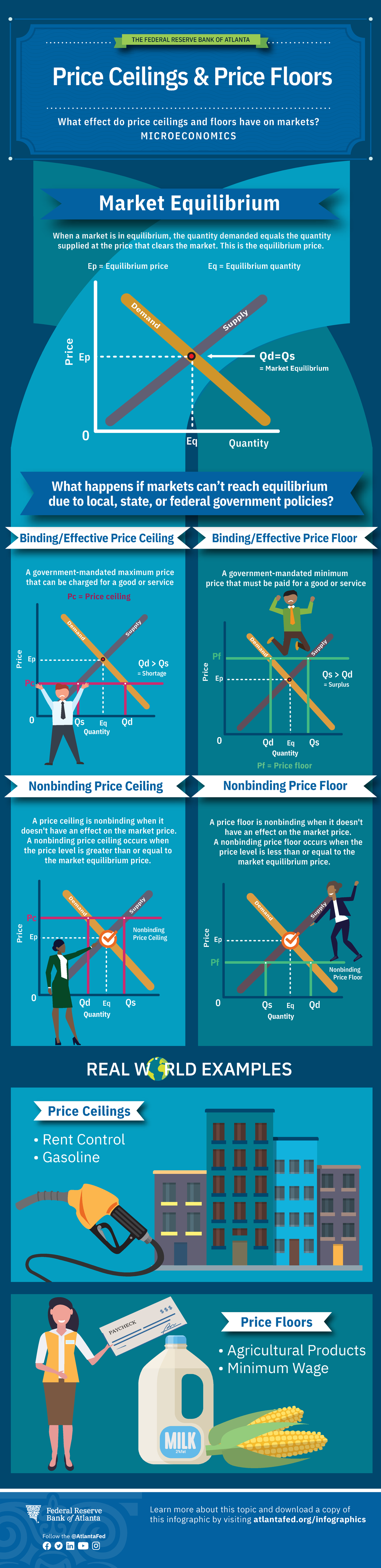
• A price ceiling is only binding (effective) if it is set below the free-market equilibrium price. If it's set above equilibrium, the market will naturally settle at the lower equilibrium price, and the ceiling will have no effect (it is non-binding).
• A price floor (which we'll cover next) is only binding if it is set above the free-market equilibrium price.

A helpful way to remember this comes from an article in Principles of Microeconomics. Think of being in a room where the walls are closing in, like the famous scene from Star Wars. You only feel constrained if the ceiling starts falling or the floor starts rising. A rising ceiling or falling floor doesn't restrict you. Similarly, only a price ceiling below equilibrium or a price floor above equilibrium is constraining, or binding.

Analyzing the Effects of a Price Ceiling

When a binding price ceiling is imposed, it creates several predictable effects. The lower price increases the quantity demanded but decreases the quantity supplied, resulting in a shortage. But what is the effect on overall welfare?

The following reading uses the common example of rent control to walk through a detailed analysis. As you read, focus on how the surplus for consumers and producers (landlords) changes and how the inefficiency, known as deadweight loss, arises.

Let's summarize the key points from the reading:

1. Shortage: At the ceiling price, quantity demanded exceeds quantity supplied.
2. Redistribution of Surplus:
   • Some consumers "win": those who can still find an apartment now pay a lower rent. Their consumer surplus increases. This is represented by a transfer of surplus from producers to consumers (Area A in the text's Figure 4.5c).
   • Producers "lose": Landlords receive lower rent for their properties, and some may exit the market altogether. Their producer surplus decreases.
   • Some consumers "lose": Other potential renters are now unable to find an apartment at all due to the shortage.
3. Deadweight Loss (DWL): Because the quantity of apartments rented is now lower than the efficient equilibrium quantity, some mutually beneficial trades no longer happen. The total economic surplus (consumer + producer) shrinks. This lost surplus is the deadweight loss, and it represents the inefficiency of the policy.

The reading makes a crucial distinction:

• The price effect of the policy causes a transfer of surplus.
• The quantity effect (the reduction in quantity traded) causes the deadweight loss.

2. Price Floors

The opposite of a price ceiling is a price floor, which is a legal minimum price. Price floors are often used in agricultural markets to support farmers' incomes or in labor markets to ensure a minimum standard of living.

Analyzing the Effects of a Price Floor

A binding price floor must be set above the equilibrium price. This high price reduces quantity demanded but increases quantity supplied, creating a surplus of the good.

To see this graphically, let's return to the Jacob Clifford video.

Application: The Minimum Wage

The most widely discussed example of a price floor is the minimum wage. In the labor market, workers are the suppliers of labor, and firms are the demanders. The "price" is the wage rate.

A minimum wage set above the equilibrium wage can lead to a surplus of labor, which we call unemployment. The quantity of labor supplied (people looking for jobs) exceeds the quantity of labor demanded (jobs offered by firms).

While the model predicts unemployment, the real-world effects of minimum wage increases are a subject of intense debate among economists. Some studies find significant unemployment effects, while others find them to be small, especially for modest increases. This is because the simple supply-and-demand model doesn't capture all the complexities of the labor market.

3. Calculating Deadweight Loss

Your background as an analyst and your preference for quantitative methods will be useful here. Being able to graphically identify deadweight loss is good, but calculating its actual value provides a more precise measure of inefficiency.

Deadweight loss is represented by a triangle on the supply and demand graph. The area of a triangle is $\frac{1}{2}\times \text{base}\times \text{height}$.

• The height of the DWL triangle is the reduction in quantity traded ($Q_{equilibrium}-Q_{control}$).
• The base of the DWL triangle is the wedge between the demand price and supply price at the new, lower quantity. For a price floor, this is the difference between the floor price and the price suppliers would have been willing to accept for that quantity.

The following video provides an excellent, step-by-step guide to performing this calculation for a price floor.

The same logic applies to calculating the deadweight loss from a price ceiling. You would find the quantity traded under the ceiling (determined by the supply curve) and then find the height of the deadweight loss triangle by looking at the price wedge at that quantity.

Practice Problem

Let's apply these concepts. Imagine the market for a product is described by the following equations:

• Demand: $P=100-2Q_D$
• Supply: $P=10+Q_S$

Part A: Find the equilibrium price and quantity.
Set the price equations equal to each other ($100-2Q=10+Q$) to solve for the equilibrium quantity $Q$, and then plug that $Q$ back into either equation to find the equilibrium price $P$.

Part B: Analyze a Price Ceiling.
Suppose the government imposes a price ceiling of $30.

1. Is this ceiling binding? Why?
2. What is the new quantity traded in the market? (Hint: at this low price, how much are firms willing to supply?)
3. Calculate the size of the shortage.

Part C: Analyze a Price Floor.
Now, suppose the government instead imposes a price floor of $60.

1. Is this floor binding? Why?
2. What is the new quantity traded in the market? (Hint: at this high price, how much are consumers willing to buy?)
3. Calculate the size of the surplus.

Conclusion

In this lesson, we moved from the idealized world of free markets to the more complex reality of government intervention. We've seen that while price controls are often implemented with good intentions—to make goods more affordable or to protect producers—they disrupt the market's signaling mechanism and lead to predictable inefficiencies.

Here are the key takeaways:

• A price ceiling is a legal maximum price. To be binding, it must be set below equilibrium. A binding ceiling causes a shortage.
• A price floor is a legal minimum price. To be binding, it must be set above equilibrium. A binding floor causes a surplus.
• Both binding price controls reduce the actual quantity of the good bought and sold in the market.
• This reduction in quantity prevents mutually beneficial trades from occurring, resulting in deadweight loss—a permanent loss of total economic surplus that signifies market inefficiency.
• Price controls also redistribute surplus. Ceilings tend to transfer surplus from producers to some consumers, while floors tend to transfer surplus from consumers to some producers.

This lesson concludes our module on the core mechanics of supply and demand. You now have a robust toolkit for analyzing how markets work and how policies affect them.

In our next module, "Consumer Choice and Utility Theory," we will take a step back and look underneath the demand curve. We'll explore the psychological and economic foundations of consumer behavior, starting with the concepts of total and marginal utility to model how individuals make choices to maximize their satisfaction. This will give you a deeper appreciation for where the demand curve comes from.