Finding Equilibrium: Graphing and Algebra

Hello! Welcome to our third lesson in the "Supply, Demand, and Market Equilibrium" module.

In our previous two lessons, we built the foundational blocks of a market. We first explored the consumer side, deriving the downward-sloping demand curve. Then, we examined the producer side, constructing the upward-sloping supply curve. So far, we have treated buyers and sellers as two separate groups.

Today, we bring them together in the same arena. This lesson is where the magic of the market happens. We will see how the independent decisions of millions of consumers and producers interact to determine the price and quantity of goods sold. Our goal is to determine equilibrium price and quantity graphically and algebraically. Mastering this is key to understanding how market-based economies allocate resources.

1. The Concept of Market Equilibrium

When we place the demand curve and the supply curve on the same graph, they will, in almost all cases, intersect at a single point. This intersection is the market equilibrium.

• The price at this intersection is called the equilibrium price, denoted as $P^{\ast }$.
• The quantity at this intersection is the equilibrium quantity, denoted as $Q^{\ast }$.

At the equilibrium price, the quantity of a good that buyers are willing and able to purchase is exactly equal to the quantity that sellers are willing and able to sell ($Q_d=Q_s$). This is a state of balance or rest; there is no inherent tendency for the market to move away from this point.

But what if the price is not at equilibrium? The market has a powerful, self-correcting mechanism. To understand this dynamic process, let's watch a video from Khan Academy.

As the video explained, any price other than the equilibrium price creates an imbalance:

• Surplus (or Excess Supply): If the market price is above $P^{\ast }$, the quantity supplied will exceed the quantity demanded ($Q_s>Q_d$). Producers are left with unsold goods. To clear their inventory, they will have an incentive to lower their prices. This downward pressure on price continues until the market reaches equilibrium.

• Shortage (or Excess Demand): If the market price is below $P^{\ast }$, the quantity demanded will exceed the quantity supplied ($Q_d>Q_s$). Too many buyers are chasing too few goods. This allows sellers to raise their prices. Also, eager buyers may bid prices up. This upward pressure on price continues until the market reaches equilibrium.

This automatic, self-correcting tendency of markets to move toward equilibrium is one of the most powerful ideas in economics.

2. Determining Equilibrium Algebraically

Visualizing the intersection on a graph is intuitive, but for precision, we turn to algebra. Given your background, you'll find this approach both familiar and powerful. The logic is simple: equilibrium occurs where quantity demanded equals quantity supplied.

Let's walk through the method with a clear example from a textbook.

Let's formalize the process you just read about. To find market equilibrium algebraically, follow these steps:

1. Start with the demand and supply equations.

   • Demand: $Q_d=a-bP$
   • Supply: $Q_s=c+dP$
     (Where $a,b,c,d$ are constants)

2. Set quantity demanded equal to quantity supplied. The condition for equilibrium is $Q_d=Q_s$.
   $a-bP=c+dP$

3. Solve for the equilibrium price ($P^{\ast }$). This involves rearranging the equation to isolate $P$.
   $a-c=bP+dP$
   $a-c=(b+d)P$
   $P^{\ast }=\frac{a-c}{b+d}$

4. Solve for the equilibrium quantity ($Q^{\ast }$). Substitute the equilibrium price ($P^{\ast }$) back into either the original demand or supply equation. You will get the same answer for $Q^{\ast }$.

   • Using the demand equation: $Q^{\ast }=a-b(P^{\ast })$
   • Using the supply equation: $Q^{\ast }=c+d(P^{\ast })$

Plugging $P^{\ast }$ into both equations is a great way to check your work. If you get different quantities, there was a mistake in the calculation for $P^{\ast }$.

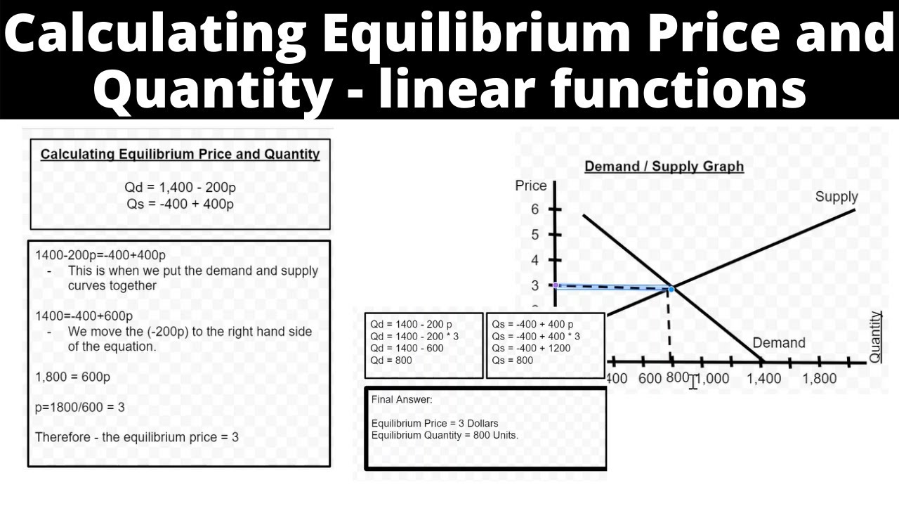
The image below shows another example, tying the algebraic steps directly to the graphical representation.

3. A Practical Application: Solving with Software

In a real-world setting, especially with more complex data or non-linear functions, economists and analysts often use software to find equilibrium. Given your work in IT, it might be interesting to see how this translates to a tool like a spreadsheet.

The core idea is the same. You can create a cell that calculates the difference between the supply and demand functions ($Q_s-Q_d$ or $P_s-P_d$). Then, you can use a solver tool (like Excel's "Goal Seek") to find the value of Q (or P) that makes this difference equal to zero.

The following resource gives a simple example of this approach.

Conclusion

Today we've reached a major milestone in the course. By combining the demand and supply models, we've seen how the independent actions of self-interested buyers and sellers are coordinated by the price mechanism to arrive at a stable market outcome.

Here are our key takeaways:

• Market Equilibrium is the point where the supply and demand curves intersect, resulting in an equilibrium price ($P^{\ast }$) and equilibrium quantity ($Q^{\ast }$).
• At equilibrium, the market "clears": quantity supplied equals quantity demanded.
• If the price is above equilibrium, a surplus will emerge, creating downward pressure on the price.
• If the price is below equilibrium, a shortage will emerge, creating upward pressure on the price.
• Equilibrium can be determined graphically by finding the intersection of the two curves.
• Equilibrium can be determined algebraically by setting the demand equation equal to the supply equation ($Q_d=Q_s$) and solving for the price.

We have now established a model of a stable market. But markets are rarely static. In our next lesson, we will use this framework as a powerful analytical tool to see what happens to price and quantity when outside events cause the demand or supply curves to shift.