Understanding and Shifting the Supply Curve

Hello! Welcome to your next lesson in our "Supply, Demand, and Market Equilibrium" module.

In the previous lesson, we thoroughly examined the buyer's side of the market by constructing the demand curve. We saw how the Law of Demand leads to a downward-sloping curve and explored the various factors that can cause that curve to shift.

Today, we will build the other half of our market model: the supply curve. This involves looking at the market from the perspective of producers and understanding what motivates their decision to sell. Many of the concepts will be parallel to what you learned about demand—such as the distinction between a movement along a curve and a shift of the curve—but the underlying logic will be entirely different.

By the end of this lesson, you will be able to plot and interpret a supply curve and identify the key factors that cause it to shift.

1. The Law of Supply and the Supply Curve

Just as demand represents consumers' willingness and ability to buy, supply represents the quantity of a good or service that producers are willing and able to sell at various prices over a given period.

This relationship between price and the quantity producers are willing to sell is governed by the Law of Supply. Let's start with a video that defines this law and shows how to represent it graphically.

As the video explained, the Law of Supply states that, ceteris paribus (all other things being equal), there is a direct relationship between the price of a good and the quantity supplied.

• As the price increases, the quantity supplied increases.
• As the price decreases, the quantity supplied decreases.

This is because a higher price increases the potential for profit, creating a powerful incentive for firms to produce and sell more. This positive relationship gives the supply curve its upward slope.

It is crucial to distinguish between two terms that sound similar:

• Supply: Refers to the entire relationship between all possible prices and quantities producers will sell. It is represented by the entire curve.
• Quantity Supplied: Refers to the specific amount producers will sell at one particular price. It is represented by a single point on the curve.

Therefore, a change in the good's own price causes a change in quantity supplied, which we see as a movement along the existing supply curve.

2. Shifts in the Supply Curve

What happens when a factor other than the good's own price changes? Just as with demand, the ceteris paribus assumption is violated, and the entire supply curve shifts.

• An increase in supply means producers are willing and able to sell more of the good at every price. This is shown as a rightward shift of the supply curve.
• A decrease in supply means producers are willing and able to sell less of the good at every price. This is shown as a leftward shift of the supply curve.

Most factors that shift the supply curve do so by changing the cost of production. If production becomes cheaper, supply increases (shifts right). If production becomes more expensive, supply decreases (shifts left).

To see this in action and learn about the specific factors that cause these shifts, let's continue with the EconplusDal video.

This video provides a great list of shifters. To deepen your understanding, the following resource from Marginal Revolution University provides a slightly different framework, emphasizing how most shifters ultimately boil down to changes in costs or opportunity costs.

3. A Summary of Supply Shifters

Let's consolidate the factors that shift the supply curve. While mnemonics are useful, your goal is to understand the logic behind each one.

For a comprehensive text-based summary and a very important clarification, please review the following resource.

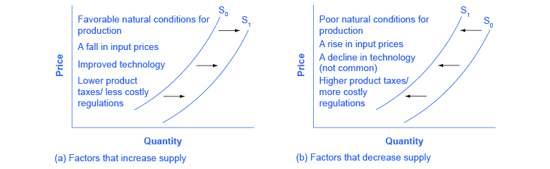
Here is a summary of the main supply shifters:

1. Prices of Inputs (Factors of Production): A decrease in the price of inputs (like labor or raw materials) lowers production costs and increases supply (shift right). An increase in input prices raises costs and decreases supply (shift left).
2. Technology: Improvements in technology lower costs and increase supply (shift right).
3. Taxes and Subsidies: Taxes on production increase costs and decrease supply (shift left). Subsidies from the government lower costs and increase supply (shift right).
4. Expectations: If firms expect prices to rise in the future, they may decrease current supply to sell more later (shift left).
5. Number of Sellers: More firms entering the market increases supply (shift right). Firms exiting the market decreases supply (shift left).
6. Prices of Alternative Goods (Opportunity Cost): If the price of an alternative product a firm could make rises, the firm may switch production to that good, decreasing the supply of the original good (shift left).
7. Natural Events: Favorable weather can increase the supply of agricultural products (shift right), while storms or droughts can decrease it (shift left).

The following image provides a great visual summary of how these factors work.

4. Application: Test Your Understanding

Let's apply these concepts. For each scenario below, decide what happens to the supply curve for gasoline. Does it shift left, shift right, or is there a movement along the curve?

1. The price of crude oil, a key input, falls dramatically.
2. The price of gasoline at the pump falls.
3. The government introduces a new tax on every liter of gasoline sold.
4. A major hurricane forces the shutdown of several large oil refineries.

---

Answers:

1. Shift right. A fall in the price of a key input (crude oil) lowers production costs. Firms are now willing to supply more gasoline at every price.
2. Movement along the curve. A change in the price of gasoline itself causes a change in quantity supplied, not a change in supply. We would move down along the existing supply curve to a lower quantity.
3. Shift left. The tax acts as an increase in the cost of production for sellers, making them willing to supply less gasoline at every price.
4. Shift left. The shutdown of refineries is equivalent to a reduction in the number of sellers (or a negative technological shock), reducing the total amount of gasoline that can be supplied at any price.

Conclusion

Excellent work. We have now built the second and final pillar of our market model. You understand how producers respond to price incentives and how their decisions are affected by a range of external factors.

Here are the key takeaways from this lesson:

• The supply curve illustrates the Law of Supply: a direct, positive relationship between a good's price and the quantity producers are willing to sell, driven by the profit motive.
• A change in the good's own price causes a movement along the supply curve (a change in quantity supplied).
• A change in a non-price factor that affects production—like input costs, technology, number of sellers, or taxes—causes a shift of the entire supply curve (a change in supply).

In our next lesson, we will bring the concepts from the last two lessons together. By plotting the demand curve and the supply curve on the same graph, we can analyze how buyers and sellers interact to determine the market equilibrium, where the price and quantity of a good are established.