Recommended resources
The freely available resources this lesson will direct you to.
- Calculating the Elasticity of Demandwww.youtube.com
- Elasticity Part 1 - PED - Professor Ryanwww.youtube.com
- Price Elasticity of Demand: Calculate & Understand Conceptswww.studypug.com
- Elasticity – Introduction to Microeconomicspsu.pb.unizin.org
- Price elasticity of demand using the midpoint method | Elasticity | Microeconomics | Khan Academywww.youtube.com
- Y1 10) Price Elasticity of Demand - PEDwww.youtube.com
Hello! In our last lesson, we saw that when supply and demand both shift, we can be certain about the direction of change for either price or quantity, but the other variable remains ambiguous. We know the market will change, but we don't know how much.
Today, we introduce a fundamental concept in economics that addresses this question of "how much": elasticity. Specifically, we will focus on the price elasticity of demand (PED). This powerful tool measures how responsive the quantity demanded of a good is to a change in its price.
Our goal for this lesson is to calculate the price elasticity of demand and interpret its value. By the end of our session, you'll be able to not only compute this crucial metric but also understand what it tells us about consumer behavior and market characteristics. This moves our analysis from being purely qualitative (direction) to quantitative (magnitude), a step that should resonate with your analytical background.
1. What is Price Elasticity of Demand?
At its core, price elasticity of demand answers a simple question: If we change the price of a product, by how much does the quantity people want to buy change?
The formal definition is:
We use percentages because they are unit-free. This allows us to compare the elasticity of very different goods—like cars and coffee—without getting bogged down in units like "cars per thousand dollars" versus "cups per cent."
To build your intuition, let's start with a short video that introduces the concept using a memorable analogy.
Price elasticity of demand using the midpoint method | Elasticity | Microeconomics | Khan Academy
This video from Khan Academy defines price elasticity of demand and uses the analogy of a rubber band to explain the difference between 'elastic' and 'inelastic' demand.
Watch the first 4 minutes and 17 seconds. Focus on why economists use percentage changes and the intuitive meaning of 'elastic' (stretchy) versus 'inelastic' (stiff) demand.
As the video explained:
- Elastic Demand: A small percentage change in price leads to a large percentage change in quantity demanded. Think of a very stretchy rubber band.
- Inelastic Demand: A large percentage change in price leads to only a small percentage change in quantity demanded. This is like a stiff, unstretchable band.
Because of the law of demand (price up, quantity demanded down), the PED will always be a negative number. However, economists often refer to its absolute value for simplicity when discussing whether it's "high" or "low."
2. How to Calculate Price Elasticity of Demand
Calculating percentage change seems straightforward: (New Value - Old Value) / Old Value. However, this "endpoint" method has a flaw: the result depends on whether the price is rising or falling. For example, the percentage change from $10 to $12 is +20%, but the change from $12 to $10 is -16.7%. This inconsistency is problematic.
To solve this, economists use the midpoint method, which calculates the percentage change relative to the average of the starting and ending values. This ensures the elasticity is the same regardless of the direction of the price change.
The midpoint formula is:
This formula may look complex, but it's just the percentage change in quantity divided by the percentage change in price, using the average as the denominator in both cases.
Let's see it in action.
Price elasticity of demand using the midpoint method | Elasticity | Microeconomics | Khan Academy
The same Khan Academy video provides an excellent, step-by-step walkthrough of a calculation using the midpoint method. Follow along closely.
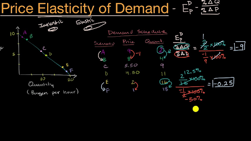
Continue watching from where you left off, from 4:17 to 9:47. The narrator will calculate the elasticity for the segment between points A and B on the demand curve. Note how he uses the average of the two quantities (3) and the average of the two prices (8.5) as the base for the calculation.
The example in the video is summarized in the image below. You can see the demand schedule (the table), the demand curve (the graph), and the resulting elasticity calculations.
Practice Calculation
Now it's your turn. Using the data from the image above and the midpoint formula, calculate the price elasticity of demand when the price of a burger falls from $4.50 (Point D) to $3.50 (Point E).
Solution:
- Identify initial and new values:
- ,
- ,
- Calculate percentage change in quantity:
- Change in Q:
- Average Q:
- %ΔQd =
- Calculate percentage change in price:
- Change in P:
- Average P:
- %ΔP =
- Calculate PED:
The price elasticity of demand for this segment is approximately -0.67.
3. Interpreting the Elasticity Value
So, we calculated a value of -0.67. What does this number actually tell us? The key lies in its absolute value.
This next short video clearly breaks down the different categories of elasticity based on the calculated value.
Y1 10) Price Elasticity of Demand - PED
This clip from EconplusDal provides a concise guide to interpreting the elasticity value you've calculated.
Watch from 1:17 to 2:46. Focus on the rules for determining if demand is elastic, inelastic, or unit elastic based on its value relative to 1.
Here is a summary of the categories of price elasticity:
| Category | Absolute Value of PED | Interpretation | Consumer Response |
|---|---|---|---|
| Perfectly Inelastic | $ | E_d | = 0$ |
| Inelastic | $0 < | E_d | < 1$ |
| Unit Elastic | $ | E_d | = 1$ |
| Elastic | $ | E_d | > 1$ |
| Perfectly Elastic | $ | E_d | = \infty$ |
In our practice problem, we found , which is less than 1. Therefore, in this price range, the demand for burgers is inelastic. A 1% drop in price leads to only a 0.67% increase in quantity demanded.
The following reading connects these numerical values to the shape of the demand curve and provides real-world examples.
This article from Penn State provides real-world context for elasticity. It connects the value of elasticity to the shape of the demand curve and lists the measured elasticities for several common goods.
Read the sections titled 'Steepness of Elasticity' and 'Summary'. Note the visual relationship: steeper demand curves are more inelastic, while flatter curves are more elastic. Also, examine the 'Some sample elasticities' list and consider why a good like gasoline has very low elasticity while movies have a high one.
As the text highlights, goods considered necessities with few substitutes (like gasoline or staple foods) tend to have inelastic demand. Consumers will buy them even if the price rises significantly. In contrast, luxuries or goods with many substitutes (like a specific brand of soda or movie tickets) tend to have elastic demand, as consumers can easily switch to an alternative if the price goes up.
Conclusion
Today, you've added a crucial quantitative tool to your economics toolkit. We've moved beyond simply saying "quantity demanded will fall" to precisely measuring by how much it will fall in percentage terms.
Here are the key takeaways from our lesson:
- Price Elasticity of Demand (PED) measures the responsiveness of quantity demanded to a price change.
- The midpoint method is the standard for calculation because it provides a consistent result regardless of the direction of the price change.
- The absolute value of PED allows us to classify demand:
- Inelastic (): Consumers are not very responsive to price changes (e.g., necessities).
- Elastic (): Consumers are very responsive to price changes (e.g., luxuries).
- Unit Elastic (): The response is proportional.
Price isn't the only factor that influences buying decisions. In our next lesson, we will expand on this concept by exploring two other types of elasticity: income elasticity, which measures how demand responds to changes in consumer income, and cross-price elasticity, which measures how the demand for one good responds to price changes in another.