Output Layer Gradient Calculation

Hello! Welcome to the fourth lesson in our "Neural Networks from Scratch" module.

In our last lesson, you successfully implemented a forward pass, allowing our network to make predictions. However, those predictions were based on random, untrained weights. To make our network intelligent, it needs a way to learn from its mistakes. This is where backpropagation comes in.

Today, we'll take the first and most crucial step in understanding this learning process. We will focus on the very last layer of the network and use calculus to figure out how sensitive the network's error is to changes in that layer's weights and biases. This sensitivity is called the gradient, and it's the key to training.

This lesson directly addresses the learning outcome: Derive the gradient of the loss function with respect to the weights and biases of the output layer.

1. From Prediction to Error: The Loss Function

Before we can correct the network's errors, we need to quantify them. We do this using a loss function (also called a cost function). This function compares the network's predictions ($\hat{y}$) with the true target values ($y$) and outputs a single number representing the total error.

A common loss function for regression tasks is the Mean Squared Error (MSE):

$$C=\frac{1}{N}\sum _{i=1}^N({\hat{y}}_i-y_i{)}^2$$

For a single training example, this simplifies to $C_0=(\hat{y}-y{)}^2$.

Our goal is to adjust the network's parameters (weights $W$ and biases $b$) to minimize this cost. The most common algorithm for this is gradient descent. The idea is to calculate the gradient of the cost function with respect to each parameter and take a small step in the opposite direction.

The update rule for any weight $W$ is:

$$W_{\text{new}}=W_{\text{old}}-\alpha \frac{\partial C}{\partial W}$$

Here, $\alpha$ is the learning rate, and $\frac{\partial C}{\partial W}$ is the gradient we need to find.

The following video provides an excellent visual intuition for gradient descent and introduces the backpropagation process we'll be exploring.

2. The Chain Rule: Deconstructing the Gradient

Now for the main task: calculating $\frac{\partial C}{\partial W^{(L)}}$ and $\frac{\partial C}{\partial b^{(L)}}$ for the final layer, which we'll call layer $L$.

To do this, we must use the chain rule from calculus. Think of the network as a chain of functions. The cost $C$ depends on the final activation $a^{(L)}$, which depends on the pre-activation $z^{(L)}$, which in turn depends on the weights $W^{(L)}$ and biases $b^{(L)}$.

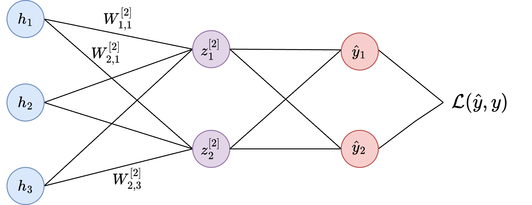
This chain of dependencies can be written as:
$C⟵a^{(L)}⟵z^{(L)}⟵W^{(L)},b^{(L)}$

The chain rule allows us to compute the overall derivative by multiplying the derivatives of each link in the chain.

A Simple Case: One Neuron Per Layer

To build intuition, let's start with the simplest possible network, where each layer has only one neuron. The 3Blue1Brown video and accompanying article are unparalleled for explaining this.

Let's formalize what you just saw. For a single training example, the cost is $C_0=(a^{(L)}-y{)}^2$. The relationships are:

1. $z^{(L)}=W^{(L)}{a}^{(L-1)}+b^{(L)}$
2. $a^{(L)}=g(z^{(L)})$, where $g$ is the activation function (e.g., sigmoid).
3. $C_0=(a^{(L)}-y{)}^2$

Gradient with respect to Weight $W^{(L)}$:
Using the chain rule, we decompose the derivative:

$$\frac{\partial C_0}{\partial W^{(L)}}=\frac{\partial C_0}{\partial a^{(L)}}\cdot \frac{\partial a^{(L)}}{\partial z^{(L)}}\cdot \frac{\partial z^{(L)}}{\partial W^{(L)}}$$

Let's compute each term:

• $\frac{\partial C_0}{\partial a^{(L)}}=2(a^{(L)}-y)$ (How much does the cost change for a small change in the final activation?)
• $\frac{\partial a^{(L)}}{\partial z^{(L)}}=g^{\prime }(z^{(L)})$ (How much does the activation change for a small change in its input? This is just the derivative of the activation function.)
• $\frac{\partial z^{(L)}}{\partial W^{(L)}}=a^{(L-1)}$ (How much does the pre-activation change for a small change in the weight? From the formula for $z^{(L)}$, we can see it's the activation of the previous neuron.)

Putting it all together:

$$\frac{\partial C_0}{\partial W^{(L)}}=2(a^{(L)}-y)\cdot g^{\prime }(z^{(L)})\cdot a^{(L-1)}$$

Gradient with respect to Bias $b^{(L)}$:
The derivation is almost identical. The first two terms of the chain rule are the same. Only the last term changes:

$$\frac{\partial z^{(L)}}{\partial b^{(L)}}=1$$

Therefore:

$$\frac{\partial C_0}{\partial b^{(L)}}=2(a^{(L)}-y)\cdot g^{\prime }(z^{(L)})\cdot 1$$

The 3Blue1Brown article provides these derivations in text form, which can be a useful reference to solidify your understanding.

3. Generalizing to Multiple Neurons (Vectorization)

The real power of neural networks comes from having multiple neurons per layer. While this introduces more indices, the core logic of the chain rule remains the same. The key is to switch from thinking about individual numbers to thinking in terms of vectors and matrices. Your background in linear algebra will be very helpful here.

Let's redefine our terms in vector form for a batch of N samples:

• $A^{(L-1)}$: Activations from the previous layer, shape (N, n_neurons_prev).
• $W^{(L)}$: Weight matrix of the output layer, shape (n_neurons_prev, n_neurons_out).
• $b^{(L)}$: Bias vector of the output layer, shape (1, n_neurons_out).
• $Z^{(L)}=A^{(L-1)}{W}^{(L)}+b^{(L)}$: Pre-activations, shape (N, n_neurons_out).
• $A^{(L)}=g(Z^{(L)})$: Final activations (predictions $\hat{Y}$), shape (N, n_neurons_out).
• $Y$: True labels, shape (N, n_neurons_out).
• $C$: Cost, a scalar.

Our goal is to find the gradient matrices $\frac{\partial C}{\partial W^{(L)}}$ (shape (n_neurons_prev, n_neurons_out)) and $\frac{\partial C}{\partial b^{(L)}}$ (shape (1, n_neurons_out)).

The following video walks through these derivations with a keen eye on the matrix dimensions, which is crucial for a correct implementation.

As the video explained, we can define an "error" term for the output layer, often denoted by delta ($\delta$). This term combines the first two parts of our chain rule:

$${\delta }^{(L)}=\frac{\partial C}{\partial Z^{(L)}}=\frac{\partial C}{\partial A^{(L)}}\odot g^{\prime }(Z^{(L)})$$

where $\odot$ denotes element-wise multiplication.

For MSE, $\frac{\partial C}{\partial A^{(L)}}=\frac{2}{N}(A^{(L)}-Y)$. So, ${\delta }^{(L)}$ becomes a matrix of shape (N, n_neurons_out).

Once we have ${\delta }^{(L)}$, the gradients are straightforward matrix operations:

• Gradient with respect to Weights $W^{(L)}$: $$\frac{\partial C}{\partial W^{(L)}}=(A^{(L-1)}{)}^T\cdot {\delta }^{(L)}$$ The shapes are (n_neurons_prev, N) dot (N, n_neurons_out), resulting in the correct gradient shape (n_neurons_prev, n_neurons_out).
• Gradient with respect to Biases $b^{(L)}$: $$\frac{\partial C}{\partial b^{(L)}}=\text{sum}({\delta }^{(L)},\text{axis}=0)$$ We sum the error contributions from all samples in the batch, resulting in a vector of shape (1, n_neurons_out).

For a more formal and compact reference, the Stanford CS224n notes provide these vectorized identities.

A very common and important special case is a classification task using a Softmax output and Cross-Entropy loss. In this specific combination, the calculation for ${\delta }^{(L)}$ simplifies beautifully to just $A^{(L)}-Y$. This is a widely used shortcut in practice.

Conclusion

Excellent work! You've tackled the most conceptually important part of backpropagation. By understanding how to calculate the gradients for the final layer, you have the starting point for the entire learning algorithm.

Key Takeaways:

• The goal of training is to minimize a loss function using an algorithm like gradient descent.
• The core of gradient descent is calculating the gradient ($\frac{\partial C}{\partial W}$) of the loss with respect to each parameter.
• We use the chain rule to break this complex derivative down into a product of simpler derivatives, following the path of computation backward from the loss.
• For the output layer $L$, the gradients are:
  • ${\delta }^{(L)}=\frac{\partial C}{\partial A^{(L)}}\odot g^{\prime }(Z^{(L)})$
  • $\frac{\partial C}{\partial W^{(L)}}=(A^{(L-1)}{)}^T\cdot {\delta }^{(L)}$
  • $\frac{\partial C}{\partial b^{(L)}}=\sum {\delta }^{(L)}$
• Expressing these operations in vectorized form is essential for efficient implementation.

In the next lesson, we will see how the error signal we just computed, ${\delta }^{(L)}$, is used to continue the process. We will propagate this error backward one more step to derive the gradient of the loss function with respect to the weights and biases of a hidden layer.