Backpropagation for Hidden Layers

Hello! Welcome to the fifth lesson in our "Neural Networks from Scratch" module.

In the last lesson, we successfully derived the gradients of the loss function for the output layer's weights and biases. We introduced the crucial "error signal" ${\delta }^{(L)}$, which represents how the final pre-activation values $Z^{(L)}$ affect the cost. This was the first step in our backward journey through the network.

Today, we take the next logical step. We will propagate that error signal one layer deeper to find the gradients for a hidden layer. This process is the core of "backpropagation" and reveals the elegant, recursive nature of the algorithm.

This lesson directly addresses the learning outcome: Apply the chain rule to derive the gradient of the loss function with respect to the weights and biases of a hidden layer.

A Quick Recap

From the previous lesson, we established the following for the final layer, $L$:

• The error signal is ${\delta }^{(L)}=\frac{\partial C}{\partial Z^{(L)}}$.
• The gradients are $\frac{\partial C}{\partial W^{(L)}}=(A^{(L-1)}{)}^T\cdot {\delta }^{(L)}$ and $\frac{\partial C}{\partial b^{(L)}}=\sum {\delta }^{(L)}$.

Our goal now is to find $\frac{\partial C}{\partial W^{(L-1)}}$ and $\frac{\partial C}{\partial b^{(L-1)}}$. To do this, we first need to find the error signal for the hidden layer, ${\delta }^{(L-1)}=\frac{\partial C}{\partial Z^{(L-1)}}$.

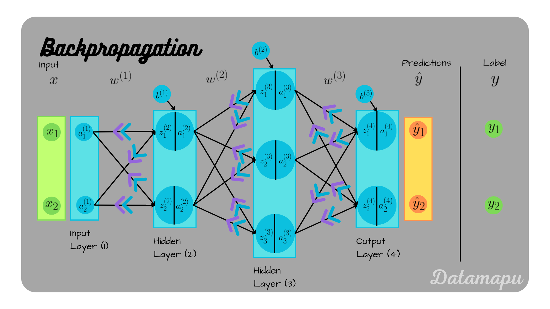
Let's look at a diagram to visualize this flow.

1. The Key Difference: A Neuron's Diverging Influence

When we considered the output layer, each neuron's activation $a_k^{(L)}$ influenced the final cost through a single, direct path.

The situation is different for a neuron in a hidden layer. A single activation in a hidden layer, say $a_j^{(L-1)}$, influences the final cost through multiple paths. It contributes to every neuron in the next layer, $L$. Each of these contributions then goes on to affect the final cost.

To correctly calculate how $a_j^{(L-1)}$ affects the cost, we must sum its influence through all these diverging paths. This is the new and most important concept for this lesson.

The following video from 3Blue1Brown provides an excellent intuition for this idea.

2. Deriving the Hidden Layer Gradients

Let's formalize the intuition from the video. We'll derive the update rules by applying the chain rule, just as before, but with an extra step to account for the diverging paths.

We want to find $\frac{\partial C}{\partial W^{(L-1)}}$. For a single weight $w_{ij}^{(L-1)}$ connecting neuron $i$ in layer $L-2$ to neuron $j$ in layer $L-1$, the chain rule gives us:

$$\frac{\partial C}{\partial w_{ij}^{(L-1)}}=\frac{\partial C}{\partial z_j^{(L-1)}}\cdot \frac{\partial z_j^{(L-1)}}{\partial w_{ij}^{(L-1)}}$$

• The second term is simple: since $z_j^{(L-1)}={\sum }_i{a}_i^{(L-2)}{w}_{ij}^{(L-1)}+b_j^{(L-1)}$, its derivative with respect to $w_{ij}^{(L-1)}$ is just $a_i^{(L-2)}$.
• The first term, $\frac{\partial C}{\partial z_j^{(L-1)}}$, is the error signal for this hidden neuron, which we'll call ${\delta }_j^{(L-1)}$.

This means $\frac{\partial C}{\partial w_{ij}^{(L-1)}}={\delta }_j^{(L-1)}{a}_i^{(L-2)}$. Our main task is to find a formula for ${\delta }_j^{(L-1)}$.

Finding the Hidden Error Signal, ${\delta }^{(L-1)}$

We apply the chain rule again to find ${\delta }_j^{(L-1)}=\frac{\partial C}{\partial z_j^{(L-1)}}$:

$${\delta }_j^{(L-1)}=\frac{\partial C}{\partial z_j^{(L-1)}}=\frac{\partial C}{\partial a_j^{(L-1)}}\cdot \frac{\partial a_j^{(L-1)}}{\partial z_j^{(L-1)}}$$

• The second term is again simple: $\frac{\partial a_j^{(L-1)}}{\partial z_j^{(L-1)}}=g^{\prime }(z_j^{(L-1)})$, the derivative of the hidden layer's activation function.
• The first term, $\frac{\partial C}{\partial a_j^{(L-1)}}$, is where we must sum the influences. The cost $C$ is affected by $a_j^{(L-1)}$ via all the neurons $k$ in the next layer, $L$.

Using the chain rule for a function with multiple intermediate variables, we get:

$$\frac{\partial C}{\partial a_j^{(L-1)}}=\sum _k\frac{\partial C}{\partial z_k^{(L)}}\frac{\partial z_k^{(L)}}{\partial a_j^{(L-1)}}$$

Let's break this down:

1. $\frac{\partial C}{\partial z_k^{(L)}}$ is simply the error signal of neuron $k$ in the output layer, ${\delta }_k^{(L)}$, which we already know how to compute from the last lesson.
2. $\frac{\partial z_k^{(L)}}{\partial a_j^{(L-1)}}$ is the rate of change of the pre-activation of neuron $k$ in layer $L$ with respect to the activation of neuron $j$ in layer $L-1$. Since $z_k^{(L)}={\sum }_j{a}_j^{(L-1)}{w}_{jk}^{(L)}+b_k^{(L)}$, this derivative is simply the connecting weight, $w_{jk}^{(L)}$.

Substituting these back gives us the crucial relationship:

$$\frac{\partial C}{\partial a_j^{(L-1)}}=\sum _k{\delta }_k^{(L)}{w}_{jk}^{(L)}$$

This means the impact of a hidden activation on the cost is the sum of the errors in the next layer, each weighted by the strength of the connection to it.

Finally, we can write the complete formula for the hidden layer error signal:

$${\delta }_j^{(L-1)}=\left(\sum _k{\delta }_k^{(L)}{w}_{jk}^{(L)}\right)g^{\prime }(z_j^{(L-1)})$$

Once we have ${\delta }_j^{(L-1)}$, the gradients for the weights and biases of the hidden layer are found using the same logic as for the output layer:

• $\frac{\partial C}{\partial w_{ij}^{(L-1)}}={\delta }_j^{(L-1)}{a}_i^{(L-2)}$
• $\frac{\partial C}{\partial b_j^{(L-1)}}={\delta }_j^{(L-1)}$ (since $\frac{\partial z_j^{(L-1)}}{\partial b_j^{(L-1)}}=1$)

This derivation is laid out very clearly in the following article.

3. Vectorization and the Total Derivative

The summation ${\sum }_k{\delta }_k^{(L)}{w}_{jk}^{(L)}$ is a clear signal that a matrix multiplication is involved. Your linear algebra background is key to understanding the elegance of the vectorized form.

Let's express our derived quantities as matrices and vectors:

• ${\delta }^{(L)}$: Error matrix for layer $L$, shape (N, n_neurons_L).
• $W^{(L)}$: Weight matrix for layer $L$, shape (n_neurons_L-1, n_neurons_L).
• $Z^{(L-1)}$: Pre-activation matrix for layer $L-1$, shape (N, n_neurons_L-1).
• $A^{(L-2)}$: Activation matrix from layer $L-2$, shape (N, n_neurons_L-2).

The summation term, which represents the backpropagated error before applying the activation derivative, becomes a matrix product:

$${\delta }^{(L)}\cdot (W^{(L)}{)}^T$$

Let's check the shapes: (N, n_neurons_L) $\cdot$ (n_neurons_L, n_neurons_L-1) results in a matrix of shape (N, n_neurons_L-1), which is exactly what we need.

This gives us the fully vectorized equation for the hidden layer error signal:

$${\delta }^{(L-1)}=({\delta }^{(L)}(W^{(L)}{)}^T)\odot g^{\prime }(Z^{(L-1)})$$

Here, $\odot$ is the element-wise (Hadamard) product.

Once we have the vectorized ${\delta }^{(L-1)}$, the gradients for the entire layer are:

• $\frac{\partial C}{\partial W^{(L-1)}}=(A^{(L-2)}{)}^T\cdot {\delta }^{(L-1)}$
• $\frac{\partial C}{\partial b^{(L-1)}}=\text{sum}({\delta }^{(L-1)},\text{axis}=0)$

Notice the beautiful recursive pattern! The formulas for the gradients are identical for every layer; only the calculation of the error signal $\delta$ changes as it propagates backward.

A Deeper Look: The Total Derivative

Given your background in math and data science, it's worth noting that this is more than just a convenient matrix operation. The use of the chain rule in this multi-path context is formally an application of the total derivative, also known as the multivariate or vector chain rule. The simple chain rule, $\frac{dy}{dx}=\frac{dy}{dt}\frac{dt}{dx}$, is a special case.

Because the cost $C$ is a function of the activations ${\mathbf{a}}^{(L)}$, which are themselves functions of the hidden activations ${\mathbf{a}}^{(L-1)}$, we are dealing with a composite function with multiple intermediate variables. The matrix multiplication ${\delta }^{(L)}(W^{(L)}{)}^T$ is the precise implementation of the total derivative required to correctly compute the gradient $\frac{\partial C}{\partial {\mathbf{a}}^{(L-1)}}$.

The following article explains this important distinction in detail.

To see these steps applied in a concrete, numerical example, the following video walks through a similar derivation component by component.

Conclusion

Fantastic work! You have now derived the complete backpropagation algorithm for a two-layer network. You've navigated the trickiest part of the derivation—understanding how to propagate the error signal from one layer to the one before it.

Key Takeaways:

• Backpropagation is a recursive algorithm where an error signal ($\delta$) is passed backward through the network.
• A hidden neuron's activation affects the cost through multiple paths, so its influence is the sum of the errors in the next layer, weighted by the connecting weights.
• The error signal for a hidden layer $l$ is calculated from the error signal of the next layer, $l+1$: ${\delta }^{(l)}=({\delta }^{(l+1)}(W^{(l+1)}{)}^T)\odot g^{\prime }(Z^{(l)})$.
• This summation is efficiently and correctly implemented as a matrix product (${\delta }^{(l+1)}(W^{(l+1)}{)}^T$), which is an application of the total derivative.
• Once ${\delta }^{(l)}$ is known, the gradient calculations for $W^{(l)}$ and $b^{(l)}$ follow the same pattern as for the output layer.

In our next lesson, we will put all this theory into practice. We'll move from equations to code and implement the full backpropagation algorithm in NumPy to compute gradients for all layers of our network.