NumPy MLP Forward Pass

Hello! Welcome to the third lesson in our module, Neural Networks from Scratch.

In our previous lessons, you learned about the individual components of a neural network: the neuron, which performs a weighted sum, and the activation functions (like ReLU, Sigmoid, and Tanh) that introduce essential non-linearity.

Today, we will assemble these pieces into a complete, functioning network. We will build a Multi-Layer Perceptron (MLP) and implement the forward pass—the core process a network uses to transform an input into a prediction. Our goal is to do this using only NumPy, which will give you a deep, fundamental understanding of the mechanics before we move to more abstract frameworks.

This lesson directly addresses the learning outcome: Implement a forward pass for a multi-layer perceptron using only NumPy.

1. The Anatomy of a Forward Pass

The "forward pass" or "forward propagation" is the flow of information from the input layer, through the hidden layers, to the output layer. At each layer, two key operations occur: a linear transformation followed by a non-linear activation.

This diagram provides an excellent visual of the process for a single input passing through a network with one hidden layer.

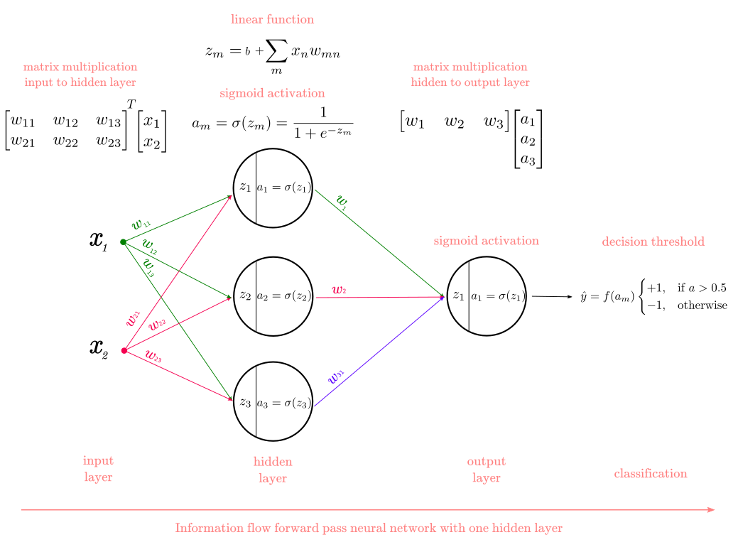
For an entire batch of data, we can express these steps efficiently using matrix operations, which is where your linear algebra background comes into play.

For any given layer $l$:

1. Linear Transformation: The pre-activation value, $Z^{[l]}$, is calculated by taking the activations from the previous layer, $A^{[l-1]}$, and multiplying them by the current layer's weight matrix, $W^{[l]}$, then adding the bias vector, $b^{[l]}$. $$Z^{[l]}=A^{[l-1]}{W}^{[l]}+b^{[l]}$$
2. Non-linear Activation: The activation for the current layer, $A^{[l]}$, is computed by applying an activation function, $g$, element-wise to $Z^{[l]}$. $$A^{[l]}=g(Z^{[l]})$$

The input data $X$ serves as the initial activation, $A^{[0]}$. This process is repeated for each layer until we reach the final output of the network.

To see this laid out in more detail, let's consult a well-written resource.

2. Implementing the Forward Pass in NumPy

Now, let's translate this theory into Python code. Our implementation will consist of two main parts: initializing the network's parameters and then defining the forward pass function itself. We will follow a fantastic video guide that builds an MLP to learn a sine function.

Initializing Network Parameters

Before we can perform a forward pass, our network needs parameters—weights and biases. These are typically stored in lists or dictionaries. The weights are initialized with small random numbers to break symmetry, while biases are often initialized to zero. More advanced initializations like Xavier or He exist to improve training stability, which the video demonstrates.

As you saw, the parameters are created based on the dimensions of consecutive layers. If we go from a layer with fan_in neurons to one with fan_out neurons, the weight matrix will have the shape (fan_in, fan_out), and the bias vector will have the shape (fan_out,).

The Forward Pass Function

With our parameters initialized, we can write the function that executes the forward pass. It will take the input data X and the parameters as arguments and return the final prediction.

3. Putting It All Together: A Complete Example

Let's synthesize what we've learned into a single, runnable code block. This example will:

1. Define the network architecture.
2. Initialize the parameters (weights and biases).
3. Implement the forward pass function.
4. Generate some dummy data and pass it through the network.

Here is the complete code, combining the concepts from the video:

import numpy as np




# Let's re-define our activation functions from the previous lesson
def sigmoid(x):
    return 1 / (1 + np.exp(-x))

def relu(x):
    return np.maximum(0, x)
    
def linear(x):



    # The 'identity' or 'linear' function for regression outputs
    return x

def initialize_parameters(layer_dims):
    """
    Initializes weights and biases for an MLP.
    
    Arguments:
    layer_dims -- python list containing the dimensions of each layer in our network
    
    Returns:
    parameters -- python dictionary containing W1, b1, ..., WL, bL
    """
    np.random.seed(42) # for reproducibility
    parameters = {}
    L = len(layer_dims) # number of layers in the network

    for l in range(1, L):



        # Xavier initialization for weights
        limit = np.sqrt(6 / (layer_dims[l-1] + layer_dims[l]))
        parameters[f'W{l}'] = np.random.uniform(-limit, limit, (layer_dims[l-1], layer_dims[l]))



        # Zero initialization for biases
        parameters[f'b{l}'] = np.zeros((1, layer_dims[l]))
        
    return parameters

def forward_pass(X, parameters, activations):
    """
    Implements a forward pass for an L-layer neural network.
    
    Arguments:
    X -- data, numpy array of shape (n_samples, n_features)
    parameters -- output of initialize_parameters()
    activations -- list of activation functions for each layer (e.g., [relu, relu, linear])
    
    Returns:
    AL -- last post-activation value (the network's prediction)
    """
    A = X
    L = len(parameters) // 2 # number of layers in the network




    # Loop from 1 to L
    for l in range(1, L + 1):
        A_prev = A
        W = parameters[f'W{l}']
        b = parameters[f'b{l}']
        



        # 1. Linear Transformation
        # Note the dimensions: (n_samples, n_features_prev) dot (n_features_prev, n_features_curr)
        Z = np.dot(A_prev, W) + b
        



        # 2. Activation
        # The activation function is selected from the list
        activation_func = activations[l-1]
        A = activation_func(Z)
        
    return A




# --- Let's test it ---




# 1. Define network architecture: 1 input feature -> 10 neurons -> 10 neurons -> 1 output
layer_dimensions = [1, 10, 10, 1]



# Define activations for each layer (hidden layers use ReLU, output uses linear for regression)
activation_functions = [relu, relu, linear]




# 2. Initialize parameters
params = initialize_parameters(layer_dimensions)




# 3. Generate some dummy input data (5 samples, 1 feature)
X_sample = np.array([[0.1], [0.5], [1.0], [1.5], [2.0]])




# 4. Perform the forward pass
predictions = forward_pass(X_sample, params, activation_functions)

print("Input data shape:", X_sample.shape)
print("Weight matrix W1 shape:", params['W1'].shape)
print("Bias vector b1 shape:", params['b1'].shape)
print("\nPredictions (output of the untrained network):")
print(predictions)
print("Predictions shape:", predictions.shape)

Run this code and examine the output. You can see how the input data of shape (5, 1) flows through the network and results in an output of shape (5, 1), as defined by our architecture. The prediction values themselves are essentially random because the network's weights have not yet been trained.

Finally, let's see this process visualized.

Conclusion

Congratulations! You have successfully implemented one of the most fundamental processes in deep learning from scratch. By translating the mathematical theory of a multi-layer perceptron into working NumPy code, you've built a solid foundation for understanding what happens inside frameworks like PyTorch and TensorFlow.

Key Takeaways:

• A forward pass is the process of making a prediction by passing input data through the network's layers.
• Each layer performs a linear transformation ($Z=AW+b$) followed by a non-linear activation ($A=g(Z)$).
• We can efficiently implement this using NumPy's np.dot() for matrix multiplication and its broadcasting capability for adding biases.
• The architecture of the network (number of layers and neurons) dictates the shapes of the weight and bias matrices.

Of course, making random predictions isn't very useful. The real power of a neural network comes from its ability to learn. In our next lesson, we will take the first step in that direction by exploring backpropagation. You will learn how to measure the network's prediction error and calculate the gradient of the loss function with respect to the weights and biases of the final layer.