The Power of Non-Linearity: Activation Functions in Deep Learning

Introduction

In our previous lesson, we established the foundational concept of the perceptron. We explored its function as a linear classifier and proved its convergence for linearly separable data. However, we concluded by identifying its critical limitation: the inability to solve non-linearly separable problems, epitomized by the XOR gate. This limitation historically stalled progress in neural network research.

This lesson directly addresses that fundamental weakness. We will explore the solution that unlocked the potential of neural networks: the introduction of non-linear activation functions. You will learn why stacking linear functions is futile and how non-linearity is the essential ingredient that allows networks of neurons to approximate arbitrarily complex patterns. We will survey the most significant activation functions—Sigmoid, Tanh, and ReLU—analyzing their mathematical properties, their historical context, and the practical trade-offs, such as the infamous vanishing gradient problem, that guide their use in modern deep learning.

The Necessity of Non-Linearity

In the last lesson, the perceptron used a simple step function. You might wonder: what if we simply stack layers of these linear units to gain more power? Let's investigate why this approach is fundamentally flawed.

A single neuron without an activation function, or with a simple linear activation $f(z)=z$, computes a linear transformation of its input: $a={\mathbf{w}}^T\mathbf{x}+b$. If we feed the output of this neuron, $a^{(1)}$, into a second linear neuron, the final output would be:

Expanding this expression gives:

If we define ${\mathbf{w}}^{\prime }={\mathbf{w}}^{(2)T}{\mathbf{w}}^{(1)T}$ and $b^{\prime }={\mathbf{w}}^{(2)T}{b}^{(1)}+b^{(2)}$, the equation simplifies to $a^{(2)}={\mathbf{w}}^{\prime T}\mathbf{x}+b^{\prime }$. This is just another linear transformation. No matter how many layers you stack, a network of purely linear units is mathematically equivalent to a single linear layer. It can only learn linear functions and is no more powerful than the simple perceptron we've already studied.

The following videos provide a concise mathematical and visual demonstration of this crucial concept.

By introducing a non-linear function $\sigma (\cdot )$ after each linear transformation, we break this chain of linearity. The output of a layer becomes $a=\sigma ({\mathbf{w}}^T\mathbf{x}+b)$. When this is fed into the next layer, the composition $\sigma ({\mathbf{w}}^{(2)T}\sigma ({\mathbf{w}}^{(1)T}\mathbf{x}+b^{(1)})+b^{(2)})$ is no longer a simple linear function. It is this non-linearity, applied layer after layer, that allows neural networks to construct highly complex, non-linear decision boundaries.

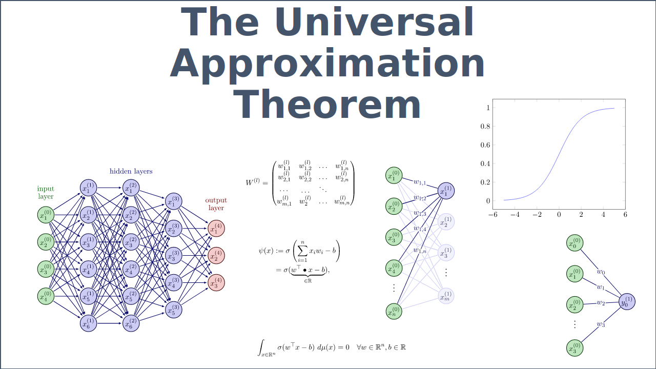
The theoretical underpinning for this is the Universal Approximation Theorem, which states that a feedforward network with a single hidden layer containing a finite number of neurons can approximate any continuous function on compact subsets of ${\mathbb{R}}^n$, under mild assumptions on the activation function. Non-linearity is the key that makes this possible.

A Tour of Activation Functions

Now that we've established the why, let's explore the what. Numerous activation functions have been proposed, each with distinct characteristics and trade-offs.

The "S"-Shaped Classics: Sigmoid and Tanh

Historically, the most popular activation functions were smooth, "S"-shaped (sigmoidal) functions. They were seen as a natural choice because their output can be interpreted as a neuron's "firing rate," smoothly transitioning from 0 (not firing) to 1 (firing at maximum rate).

As the paper discusses, both Sigmoid and Tanh have a critical flaw: their gradients become extremely small in the saturated regions (where the input is large positive or large negative). The derivative of the sigmoid function, ${\sigma }^{\prime }(x)=\sigma (x)(1-\sigma (x))$, has a maximum value of only 0.25 at $x=0$ and approaches zero as $|x|\to \infty$.

During backpropagation (which we will detail in a future lesson), the gradient of the loss is multiplied by the gradient of the activation function at each layer. If these gradients are consistently small numbers (less than 1), their product across many layers will shrink exponentially, "vanishing" to near zero. This means the neurons in the early layers of a deep network receive almost no update signal, and learning grinds to a halt.

The Modern Workhorse: Rectified Linear Unit (ReLU)

The vanishing gradient problem severely limited the depth of networks that could be effectively trained. The solution came from a surprisingly simple function: the Rectified Linear Unit, or ReLU.

ReLU is defined as:

Its derivative is also simple: 1 for $x>0$ and 0 for $x\le 0$.

This function has several key advantages:

1. Combats Vanishing Gradients: For positive inputs, the gradient is a constant 1. This means gradients can pass backward through active neurons without shrinking, allowing for much deeper networks to be trained effectively.
2. Computational Efficiency: Both the function and its derivative are trivial to compute, unlike the exponentials in Sigmoid and Tanh.
3. Sparsity: For any given input, many ReLU neurons will have a negative pre-activation value and thus an output of 0. This "sparsity" in activations can make the network more efficient and has been argued to be beneficial for learning disentangled representations.

However, ReLU is not without its own problems.

The "dying ReLU" problem occurs when a neuron's weights are updated in such a way that its pre-activation value becomes consistently negative for all data points in the training set. Since the gradient is 0 for negative inputs, the neuron's weights will never be updated again. It becomes "dead," contributing nothing to the network's output.

To address this, several variants have been proposed:

• Leaky ReLU: $f(x)=\max (\alpha x,x)$, where $\alpha$ is a small constant like 0.01. This introduces a small, non-zero gradient for negative inputs, preventing neurons from dying completely.
• Parametric ReLU (PReLU): The slope $\alpha$ is treated as a learnable parameter for each neuron.
• Exponential Linear Unit (ELU): Uses a curved function for negative values, which can help push mean activations closer to zero, similar to Tanh.

These variants ensure that there is always some gradient flow, making the network more robust.

Practical Considerations and Recommendations

The choice of activation function is a key element of neural network design. The transition from Sigmoid/Tanh to ReLU and its variants was a major catalyst for the deep learning revolution.

The review paper you've been reading concludes with a practical comparison and a set of useful heuristics.

The general consensus in modern practice is:

• Start with ReLU as your default choice for hidden layers. It is fast and generally works very well.
• If you observe a large number of "dead" neurons in your network, switch to Leaky ReLU or another variant like ELU.
• Sigmoid is still commonly used in the output layer for binary classification problems, as its (0, 1) range is perfect for representing a probability.
• Tanh can sometimes be effective in recurrent neural networks (RNNs) due to its zero-centered nature, but has largely been superseded by more advanced architectures.

Conclusion

In this lesson, we have uncovered the critical role of non-linearity in empowering neural networks. We have seen how it breaks the limitations of linear models, enabling the approximation of complex, real-world functions.

Here are the key takeaways from our exploration:

• Non-Linearity is Essential: A neural network with purely linear activation functions is no more powerful than a single linear model, regardless of its depth. Non-linearity is the key to learning complex patterns.
• Sigmoid and Tanh: These "S"-shaped functions were historical mainstays but suffer from the vanishing gradient problem, which limits their effectiveness in deep networks.
• ReLU: The modern default activation for hidden layers. It is computationally efficient and solves the vanishing gradient issue for positive inputs but can suffer from the "dying ReLU" problem.
• ReLU Variants: Leaky ReLU and other variants provide a small, non-zero gradient for negative inputs, making them more robust against dying neurons.
• A Practical Choice: The selection of an activation function is a design trade-off. ReLU is a strong starting point, with its variants offering a solution to its primary weakness.

We have now defined a neuron model—a linear transformation followed by a non-linear activation—that can serve as a powerful building block. In the next lesson, we will assemble these blocks to construct a full feedforward neural network and define its forward propagation mechanism mathematically, laying the groundwork for understanding how these models make predictions.