Building and Propagating Feedforward Networks

Introduction

In our last session, we investigated the critical role of non-linear activation functions. We saw that they are the essential ingredient that allows a network of neurons to escape the limitations of linear models and learn complex, non-linear patterns. We now have the fundamental building block: a neuron that computes a weighted sum of its inputs, adds a bias, and then passes the result through a non-linear activation function.

This lesson takes the logical next step. We will assemble these individual neurons into a structured, multi-layered architecture known as a feedforward neural network. You will learn to construct these networks by defining their layers—input, hidden, and output. Then, we will precisely define the mathematical process of forward propagation, the mechanism by which an input signal flows through the network to produce a final prediction. This process is the foundation for everything that follows, as a network must first be able to make a prediction before it can learn from its errors.

Constructing a Feedforward Neural Network

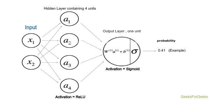
A feedforward neural network (FFNN), also called a multi-layer perceptron (MLP), is organized into a series of layers. Information flows in one direction—forward—from the input layer, through one or more hidden layers, to the output layer. There are no cycles or feedback loops, hence the name "feedforward."

The core components are:

• Input Layer: This layer represents the input features of your data. It doesn't perform any computation; it simply passes the raw input values ($\mathbf{x}$) to the first hidden layer. The number of neurons in this layer is equal to the dimensionality of the input data (e.g., the number of pixels in an image or the number of features in a dataset).
• Hidden Layers: These are the layers between the input and output. Each neuron in a hidden layer is a computational unit as we defined it in the last lesson. These layers are "hidden" because they have no direct connection to the outside world—their inputs come from the previous layer, and their outputs go to the next. The magic of deep learning happens here; as data passes through successive hidden layers, the network learns increasingly abstract and complex features.
• Output Layer: This is the final layer of the network. It produces the model's prediction, $\hat{\mathbf{y}}$. The number of neurons and the activation function used in this layer depend on the task. For regression, it might be a single neuron with a linear activation. For binary classification, it could be a single neuron with a sigmoid activation. For multi-class classification, it's typically a layer with one neuron per class, using a softmax activation.

A common architectural choice is to make the layers fully-connected (or dense), meaning every neuron in one layer is connected to every neuron in the next.

The video below offers an excellent conceptual walkthrough, illustrating how we move from a single neuron (logistic regression) to a full multi-layer network and introduces the powerful idea that hidden layers learn a hierarchy of features.

The number of hidden layers and the number of neurons in each are key hyperparameters of the model—structural choices you make before training begins.

The Mathematics of Forward Propagation

Forward propagation is the computational process of passing an input vector $\mathbf{x}$ through the network, layer by layer, to generate a prediction $\hat{\mathbf{y}}$. At each layer $l$, two steps are performed for each neuron:

1. Compute the weighted sum (pre-activation): A linear transformation of the activations from the previous layer, ${\mathbf{a}}^{[l-1]}$. We denote this intermediate value as ${\mathbf{z}}^{[l]}$.
2. Apply the non-linear activation function: Pass ${\mathbf{z}}^{[l]}$ through a non-linear function $g^{[l]}(\cdot )$ (like ReLU) to get the final output of the layer, ${\mathbf{a}}^{[l]}$.

This process is repeated until we reach the output layer.

Formal Definition

Let's define this process with mathematical rigor. The following article provides a clear, step-by-step derivation, which is ideal given your background in computer science and mathematics. It starts with the scalar form and builds up to the fully vectorized form used in practice.

To make this tangible, let's trace the flow of data through a concrete example.

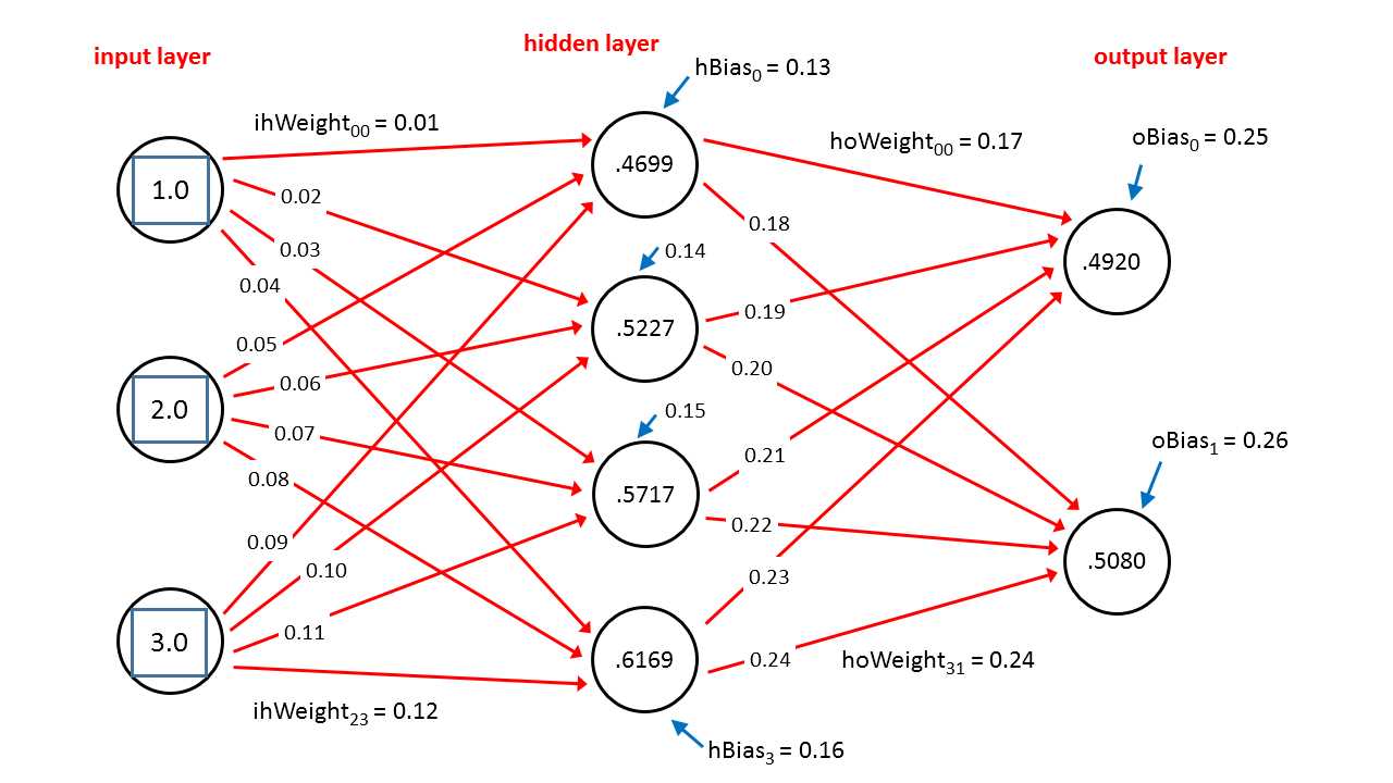
Let's verify the calculation for the top neuron in the hidden layer. Its pre-activation value, $z_0^{[1]}$, is the weighted sum of the inputs plus its bias.

• Inputs (${\mathbf{a}}^{[0]}$): [1.0, 2.0, 3.0]
• Weights to this neuron (${\mathbf{W}}_{0,:}^{[1]}$): [0.01, 0.05, 0.09]
• Bias for this neuron ($b_0^{[1]}$): 0.13

The pre-activation $z_0^{[1]}$ is computed as:

The final activation, $a_0^{[1]}$, is then calculated by applying the layer's activation function, $g^{[1]}$, to this value: $a_0^{[1]}=g^{[1]}(0.51)$. The diagram shows a result of 0.4699. (Note: this specific value results from an unstated activation function, but the two-step process of weighted sum then activation is the key takeaway). This same procedure is repeated for every neuron in the hidden layer, and then again for the output layer using the hidden layer's activations as input.

From a Single Example to a Batch: Vectorization

In any real-world application, you will process thousands or millions of training examples. Performing forward propagation one example at a time is computationally inefficient. The true power and speed of modern deep learning frameworks come from vectorization—processing an entire "batch" of inputs simultaneously using matrix operations.

Instead of an input vector $\mathbf{x}$, we have an input matrix $\mathbf{X}$, where each column is a separate training example. The forward propagation equations are updated to operate on these matrices.

The equation for a layer becomes:

Here, ${\mathbf{A}}^{[l-1]}$ is a matrix where each column is the activation vector from the previous layer for one example in the batch. Now, consider the dimensions. If layer $l$ has $n^{[l]}$ neurons, layer $l-1$ has $n^{[l-1]}$ neurons, and we have a batch of $m$ examples:

• ${\mathbf{W}}^{[l]}$ has shape $(n^{[l]},n^{[l-1]})$.
• ${\mathbf{A}}^{[l-1]}$ has shape $(n^{[l-1]},m)$.
• The product ${\mathbf{W}}^{[l]}{\mathbf{A}}^{[l-1]}$ results in a matrix of shape $(n^{[l]},m)$.
• The bias ${\mathbf{b}}^{[l]}$ is a vector of shape $(n^{[l]},1)$.

This leads to a classic linear algebra problem: adding a matrix of shape $(n^{[l]},m)$ to a vector of shape $(n^{[l]},1)$. This is resolved through a mechanism called broadcasting. The bias vector ${\mathbf{b}}^{[l]}$ is implicitly duplicated $m$ times to form a matrix of shape $(n^{[l]},m)$, allowing for element-wise addition. Your familiarity with computational libraries like NumPy makes this concept very natural, as broadcasting is a fundamental feature of their design.

This short video explains the transition to batch processing and the concept of broadcasting with exceptional clarity.

The final step is to apply the activation function element-wise to the matrix ${\mathbf{Z}}^{[l]}$ to get the activation matrix ${\mathbf{A}}^{[l]}$, which then becomes the input for the next layer. This fully vectorized process is the engine of forward propagation in all modern deep learning frameworks.

Conclusion

In this lesson, we have moved from the single neuron to a complete, functioning feedforward neural network. We defined the architectural components and, most importantly, detailed the mathematical engine of forward propagation that allows the network to generate predictions.

The key takeaways are:

• Architecture: Feedforward networks are built from an input layer, one or more hidden layers, and an output layer. In fully-connected networks, every neuron in a layer is connected to every neuron in the subsequent layer.
• Forward Propagation: This is the process of computing a prediction by passing input data through the network. It consists of a sequence of layer-wise operations: a linear transformation (weighted sum + bias) followed by a non-linear activation.
• Mathematical Formulation: For a layer $l$, the core computation is ${\mathbf{a}}^{[l]}=g({\mathbf{W}}^{[l]}{\mathbf{a}}^{[l-1]}+{\mathbf{b}}^{[l]})$, where ${\mathbf{a}}^{[0]}$ is the input $\mathbf{x}$.
• Vectorization: Processing a batch of $m$ examples at once is achieved by stacking inputs into matrices (e.g., $\mathbf{X}$ of size $n_{features}\times m$). The bias vector is added to the result of the matrix multiplication via broadcasting.

We now have a complete description of how a neural network produces an output from an input, given a set of weights and biases. However, we have not yet discussed how the network finds the correct values for these parameters. This is the task of training. In our next lesson, we will introduce the concept of a loss function and then derive the backpropagation algorithm, the recursive application of the chain rule that allows the network to compute the gradients needed to learn its parameters.