Perceptron Model: Limitations and Linearly Separable Problems

Recommended resources

The freely available resources this lesson will direct you to.

Introduction

Welcome to our first lesson on the foundations of deep neural networks. In the previous module, we concluded our exploration of unsupervised learning by examining t-SNE, a powerful technique for visualizing high-dimensional data. We saw how it focuses on preserving local neighborhood structures, offering a different perspective from methods like PCA which preserve global variance.

Now, we pivot from discovering latent structure to building models that learn to make predictions—the domain of supervised learning, which forms the bedrock of modern AI. Our journey begins with the simplest component of a neural network, a historical and conceptual building block known as the perceptron. In this lesson, you will learn the mathematical definition of the perceptron model, understand its function as a linear classifier, and, most importantly, grasp its fundamental limitation to linearly separable problems, which historically motivated the development of the more complex networks we use today.

The Perceptron Model: A Simple Computational Neuron

The perceptron, developed by Frank Rosenblatt in the late 1950s, was one of the first formal models of an artificial neuron capable of learning. It draws inspiration from biological neurons, which receive signals, integrate them, and "fire" an output if a certain threshold is exceeded.

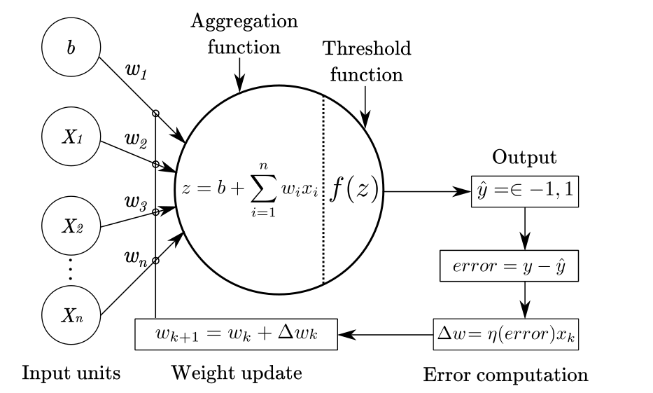
A perceptron formalizes this process mathematically. It takes a set of numerical inputs, computes a weighted sum of these inputs, adds a bias term, and passes the result through a step function to produce a binary output.

Perceptron | Neural Networks

To start, watch this brief segment from First Principles of Computer Vision. It provides a clear visual and mathematical introduction to the perceptron's components: inputs, weights, bias, and the step activation function.

Watch from the beginning to the mathematical model. This will give you a concise overview of the perceptron's operation.

As the video explained, for a set of inputs $x = [x_{1}, x_{2}, \dots, x_{n}]^{T}$ and a corresponding set of weights $w = [w_{1}, w_{2}, \dots, w_{n}]^{T}$ , the perceptron first computes the net input, $z$ :

z = i = 1 \sum n w_{i} x_{i} + b = w^{T} x + b

Here, $b$ is the bias term. The output, $y^$ , is then determined by an activation function, which for a classic perceptron is a simple step function (or Heaviside step function):

y^= f (z) = {10 if z > 0 otherwise

(Note: Sometimes the threshold is at 0, and outputs are {0, 1} or {-1, 1}. The core principle remains the same.)

The weights $w_{i}$ determine the importance of each input $x_{i}$ . The bias $b$ can be thought of as adjusting the "firing threshold" of the neuron, making it easier or harder to output a 1.

This diagram illustrates the full structure of a single perceptron. Inputs $(X_1, ..., X_n)$ are multiplied by weights $(w_1, ..., w_n)$ and summed with a bias $b$. The result, $z$, is passed through a threshold function $f(z)$ to produce an output $\hat{y}$. The diagram also shows the mechanism for learning, which we will discuss shortly.

Geometric Interpretation: The Linear Classifier

The true power of the perceptron lies in its geometric interpretation. The equation for the decision boundary, where the net input $z$ is exactly zero, is:

w^{T} x + b = 0

For a two-dimensional input $x = [x_{1}, x_{2}]^{T}$ , this equation becomes $w_{1} x_{1} + w_{2} x_{2} + b = 0$ , which you'll recognize as the equation of a line. In $n$ -dimensional space, this defines a hyperplane.

This hyperplane divides the input space into two half-spaces:

For any point $x$ on one side of the hyperplane, $w^{T} x + b > 0$ , and the perceptron outputs 1.
For any point on the other side, $w^{T} x + b \leq 0$ , and the perceptron outputs 0.

Thus, a perceptron is fundamentally a linear classifier. The weight vector $w$ is always normal (orthogonal) to the decision boundary and points into the half-space for the positive class (output 1). The bias $b$ effectively shifts the hyperplane parallel to itself without changing its orientation.

The following reading explains this concept using the logical AND gate as a concrete example of a problem that can be solved by a perceptron.

4 Perceptron Learning Rule

This excerpt from a textbook chapter provides a detailed, formal explanation of the perceptron's architecture and its geometric interpretation as a decision boundary.

Please read the section titled "Single-Neuron Perceptron". It starts with a generic two-input example and then walks through the design of a perceptron that solves the AND gate, a classic example of a linearly separable problem. Focus on how the equation for the boundary defines a line, and how the weights and bias are chosen to correctly classify the inputs.

Learning and the Perceptron Convergence Theorem

So far, we have seen what a perceptron is. But its most revolutionary feature was its ability to learn the appropriate weights and bias from data. The process is remarkably simple and is based on error correction. This is the Perceptron Learning Rule:

Initialize weights $w$ and bias $b$ with small random values.
For each training example $(x, y)$ , where $y$ is the true label:
a. Calculate the perceptron's output $y^$ .
b. If the output is correct ( $y^= y$ ), do nothing.
c. If the output is incorrect, update the weights and bias.

The update rule is:

w_{new} = w_{old} + η (y - y^) x

b_{new} = b_{old} + η (y - y^)

Here, $η$ (eta) is the learning rate, a small positive constant that controls the size of the updates. The term $(y - y^)$ will be either +1 or -1 (assuming labels {0,1}), determining the direction of the update. The intuition is to nudge the decision boundary to correctly classify the misclassified point.

This simple algorithm comes with a powerful guarantee, formalized in the Perceptron Convergence Theorem. It states that if a dataset is linearly separable, the perceptron learning algorithm is guaranteed to find a set of weights and bias that perfectly separates the data in a finite number of updates.

Given your background, you will likely appreciate the elegance of the proof for this theorem. It's a classic result in machine learning theory.

Lecture 6 "Perceptron Convergence Proof" -Cornell CS4780 SP17

This video from a Cornell CS course provides a complete, step-by-step proof of the Perceptron Convergence Theorem. The instructor, Kilian Weinberger, does an excellent job of building the mathematical intuition.

The proof builds in four key stages. I recommend watching them in order: Setup and Assumptions: This part establishes the notation and necessary simplifying assumptions, such as the existence of a separating hyperplane \mathbf{w}^* and the normalization of data. Growth of the Inner Product: This is the first key insight. It shows that with every mistake, the inner product \mathbf{w}^T \mathbf{w}^* increases by at least a constant amount (\gamma, the margin). This means our weight vector \mathbf{w} gets more aligned with the ideal solution \mathbf{w}^*. Bounded Growth of the Norm: This second insight shows that the squared norm of our weight vector, \|\mathbf{w}\|^2, does not grow uncontrollably. It increases by at most a constant value with each mistake. Putting it Together: By combining the lower bound from step 2 and the upper bound from step 3 using the Cauchy-Schwarz inequality, the proof derives an upper bound on the total number of mistakes the algorithm can make, M \le 1/\gamma^2. Since this number is finite, the algorithm must converge.

The Perceptron's Limitation: The XOR Problem

The convergence theorem is powerful, but it contains a critical condition: "if a dataset is linearly separable." What happens if it's not?

This is the perceptron's fundamental weakness. It can only learn linear decision boundaries. Any problem that cannot be solved by drawing a single hyperplane is beyond the capability of a single perceptron. The classic, canonical example of such a problem is the XOR (exclusive OR) logical function.

The XOR function takes two binary inputs and outputs 1 if the inputs are different, and 0 if they are the same:

(0, 0) -> 0
(0, 1) -> 1
(1, 0) -> 1
(1, 1) -> 0

If you plot these four points on a 2D plane, you will find it impossible to draw a single straight line that separates the points labeled '1' from the points labeled '0'.

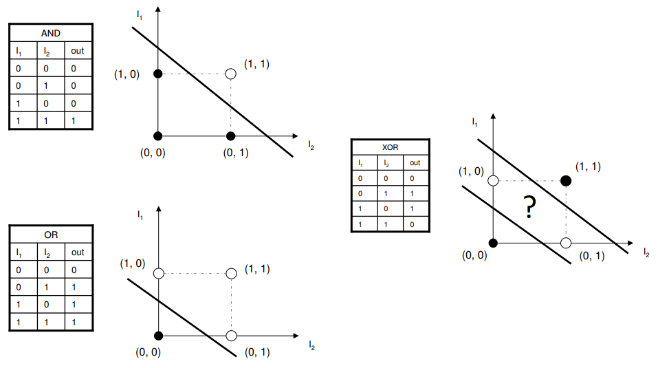
This image graphically demonstrates the concept of linear separability. The AND and OR functions are linearly separable; a single line can separate the positive cases (white circles) from the negative cases (black circles). The XOR function, however, is not linearly separable, as no single line can achieve this separation.

This limitation, famously highlighted in the 1969 book Perceptrons by Marvin Minsky and Seymour Papert, had a profound historical impact. It showed that this promising model of computation had severe limitations, contributing to a period of reduced funding and interest in neural network research, often called the first "AI winter."

4 Perceptron Learning Rule

Let's return to the textbook chapter to formalize this limitation.

Read the section titled "Limitations". It begins by defining linear separability and then immediately introduces the XOR problem with its graphical representation. The summary that follows succinctly states the main result: single-layer perceptrons can only classify linearly separable vectors.

Conclusion

In this lesson, we have taken our first step into the world of neural networks by dissecting its most elementary component, the perceptron. You've seen that it's a simple yet elegant model of a computational neuron that functions as a linear classifier.

Here are the key takeaways:

The Perceptron Model: It computes a weighted sum of its inputs, adds a bias, and uses a step function to produce a binary output.
Geometric View: A perceptron creates a hyperplane in the input space that serves as a linear decision boundary, separating the data into two classes.
Learning and Convergence: The Perceptron Learning Rule updates weights to correct mistakes. The Perceptron Convergence Theorem guarantees it will find a solution in a finite number of steps, but only if the data is linearly separable.
Fundamental Limitation: The perceptron's inability to solve non-linearly separable problems, famously exemplified by the XOR gate, is its critical weakness.

This very limitation is what drives us forward. How can we build models that learn non-linear decision boundaries? The answer lies in moving beyond a single step function. In our next lesson, we will explore the crucial role of non-linear activation functions. By replacing the perceptron's simple step function with smoother, non-linear alternatives like Sigmoid, Tanh, and ReLU, we unlock the ability to stack layers of neurons, forming the deep networks that can learn the complex patterns that the perceptron cannot.