Deriving the Volumetric Rendering Equation

Recommended resources

The freely available resources this lesson will direct you to.

Welcome to the next stage of our journey into Neural Radiance Fields. In our last lesson, we tackled the representation problem. We discovered that a standard MLP suffers from spectral bias, making it incapable of learning the high-frequency details needed for photorealism. We then derived the solution: positional encoding using Fourier features, which transforms the input coordinates to enable the network to capture detail at multiple scales.

We now have an MLP, which we can denote as $F_{θ} : (x, d) \to (c, σ)$ , that can predict the color $c$ and volume density $σ$ for any 3D point $x$ viewed from a direction $d$ . But this is just a function. How do we get from this continuous 3D representation to a final 2D image?

This lesson answers that question by focusing on the rendering process. We will derive the classical volumetric rendering equation from the first principles of light transport. This equation is the mathematical bridge that allows us to query our neural representation along a camera ray and accumulate the results to synthesize the color of a single pixel.

The Physics of Light in a Participating Medium

Before we write down any equations, let's build an intuition for what happens when a ray of light travels through a "participating medium" — a volume that is not empty space, but filled with tiny particles, like smoke, fog, or dust.

Imagine you are looking through a cloud of smoke. The light that reaches your eye is a combination of several effects:

Absorption: Particles in the smoke absorb some of the light, making things behind the smoke appear dimmer.
Emission: If the smoke is from a fire, the hot particles may glow, adding light along your line of sight.
Scattering: Light can be deflected by particles. This has two components:
- Out-scattering: Light that was originally traveling towards your eye hits a particle and is scattered away in a different direction. Like absorption, this reduces the light you see.
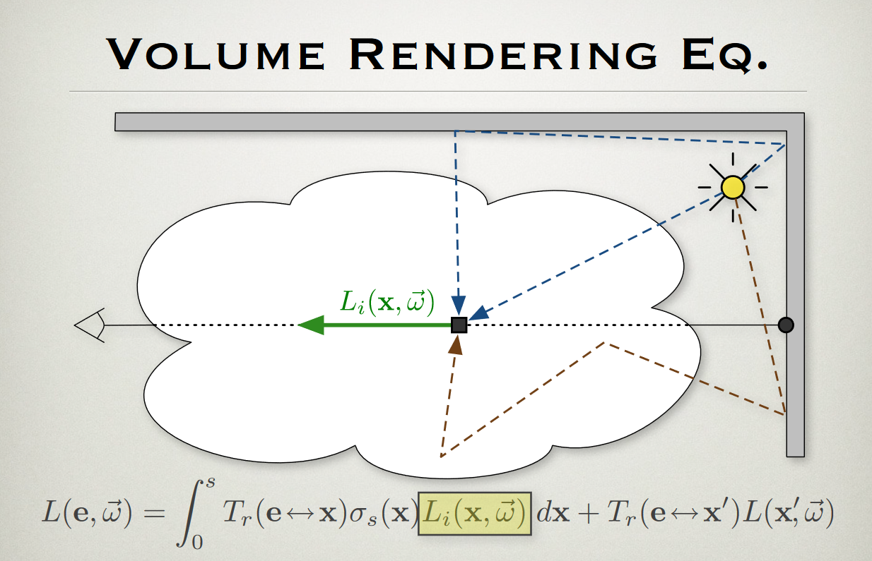
- In-scattering: Light from other sources (e.g., a lightbulb off to the side) hits a particle and is scattered into your line of sight. This adds light.

The following video provides an excellent overview of these four phenomena.

Interactive Graphics 25 - Volume Rendering

This video from Cem Yuksel's Interactive Graphics course, which you're familiar with, introduces the core interactions between light and a volumetric medium.

Watch the segment from light interaction phenomena. As you watch, focus on categorizing each effect as either a loss of light (attenuation) or a gain of light (source) along the ray's path.

These physical interactions are captured by a powerful differential equation known as the Radiative Transport Equation (RTE). It describes the change in radiance (light intensity) as a function of distance traveled through the medium.

From Physics to a Differential Equation

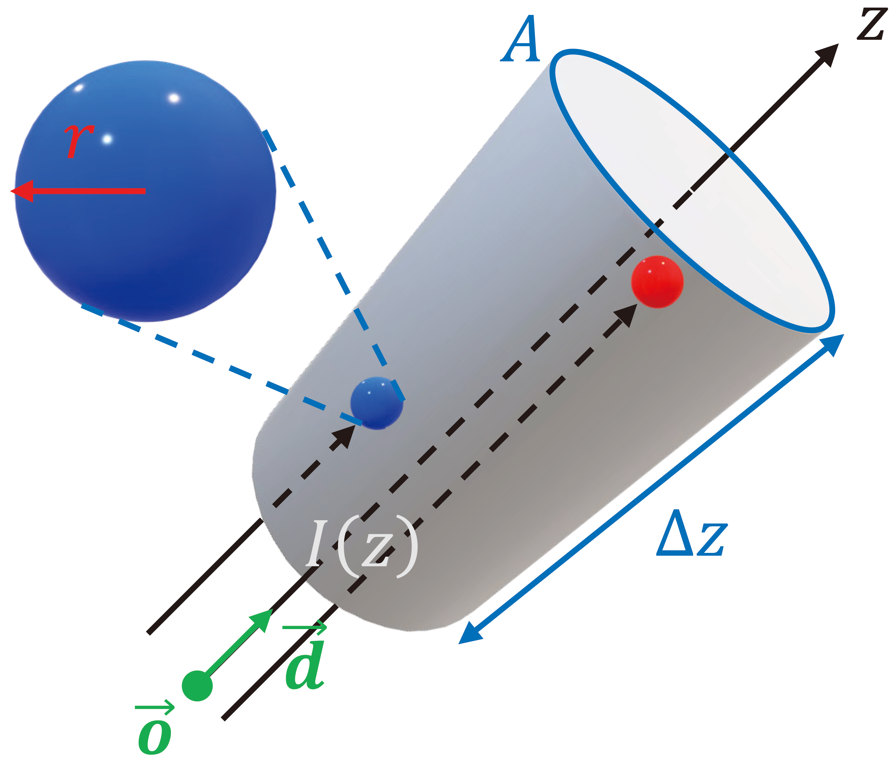
Let's formalize the intuition we just built. Consider a single camera ray $r (z) = o + z d$ , where $o$ is the camera origin, $d$ is the ray direction, and $z$ is the distance along the ray. Let $L (z)$ be the radiance (light energy) traveling along this ray at distance $z$ .

We want to find $\frac{d L ( z )}{d z}$ , the rate of change of radiance as the ray moves through the medium.

Attenuation (Loss): Both absorption and out-scattering cause a loss of radiance. This loss is proportional to how much radiance is currently present, $L (z)$ , and how dense the medium is at that point. We combine these two effects into a single term called the extinction coefficient, $σ (z)$ . In the context of NeRF, this is simply called the volume density. The change due to attenuation over an infinitesimal distance $d z$ is:
$d L_{l oss} = - σ (z) L (z) d z$
Source (Gain): Both emission and in-scattering add radiance. We can model this as a source term $S (z)$ that represents the amount of light added per unit distance. The change due to this source term is:
$d L_{g ain} = S (z) d z$

Combining these gives the Radiative Transport Equation:

\frac{d L ( z )}{d z} = L^{'} (z) = S (z) - σ (z) L (z)

This equation states that the change in radiance at any point is the sum of what's added by the source term minus what's lost to attenuation.

The following video provides a concise and formal introduction to the RTE, framing it in the context of astrophysics, which offers a rigorous first-principles perspective.

Radiative Transport Equation: Moving Energy on the Photon Train

This video by Aaron Parsons from UC Berkeley introduces the Radiative Transport Equation as a fundamental tool for understanding how energy moves through a medium.

Watch the first two segments, covering the setup and the equation itself. Note that the notation is slightly different: s is used for distance, I_\nu for specific intensity (radiance), j_\nu for emission, and \alpha_\nu for the extinction coefficient. You can map these directly to our z, L(z), source term S(z), and density \sigma(z).

Deriving the Integral Solution: The Volume Rendering Equation

We now have a differential equation. To find the total light that reaches the camera, we need to solve it. Let's do this in two steps.

Step 1: Solving for Attenuation and Defining Transmittance

First, let's consider the simplest case: a medium with only attenuation ( $S (z) = 0$ ). The RTE simplifies to:

\frac{d L ( z )}{d z} = - σ (z) L (z)

Socratic Question: Given your calculus background, this is a separable ordinary differential equation. How would you solve for $L (z)$ in terms of its initial value $L (z_{n})$ at a starting point $z_{n}$ ?

...

By separating variables, we get $\frac{d L}{L} = - σ (z) d z$ . Integrating both sides from a starting point $z_{n}$ to a point $z$ gives:

\int_{L (z_{n})}^{L (z)} \frac{1}{L ^{'}} d L^{'} = - \int_{z_{n}}^{z} σ (s) d s

ln (L (z)) - ln (L (z_{n})) = - \int_{z_{n}}^{z} σ (s) d s

L (z) = L (z_{n}) exp (- \int_{z_{n}}^{z} σ (s) d s)

This solution introduces a critical concept: Transmittance. We define the transmittance from point $a$ to point $b$ as:

T (a \to b) = exp (- \int_{a}^{b} σ (s) d s)

Transmittance, $T$ , is a value between 0 and 1 representing the fraction of light that survives the journey from $a$ to $b$ . It can be interpreted as the probability that a photon travels this path without interacting with any particles.

This derivation is laid out very clearly in the following document.

[PDF] Volume Rendering Digest (for NeRF)

This document provides a concise mathematical derivation of the key components of the volume rendering equation.

Read the first section on Transmittance. This formalizes the derivation we just completed.

Step 2: The Full Integral Equation

Now, let's incorporate the source term. In NeRF, we make a physical assumption: light is "emitted" only when a ray hits a particle. The probability of a ray hitting a particle over an infinitesimal distance $d z$ is $σ (z) d z$ . If a hit occurs, the particle emits light of color $c (z)$ . Therefore, the source term is not independent but is given by $S (z) = c (z) σ (z)$ .

The radiance that reaches the camera from a single point $z$ on the ray is the light emitted at that point, $c (z) σ (z) d z$ , multiplied by the transmittance from that point back to the camera's near plane ( $z_{n}$ ).

d C = T (z_{n} \to z) \cdot c (z) σ (z) d z

To get the final pixel color $C (r)$ , we must sum (integrate) these contributions from all points along the ray, from the near plane $z_{n}$ to the far plane $z_{f}$ .

A camera ray with origin **o** and direction **d** passing through a volumetric medium. The final color is an integral of contributions from points along the segment from z_near to z_far.

This gives us the classical volume rendering equation:

C (r) = \int_{z_{n}}^{z_{f}} T (z_{n} \to z) σ (r (z)) c (r (z), d) d z

where the transmittance is defined as before:

T (z_{n} \to z) = exp (- \int_{z_{n}}^{z} σ (r (s)) d s)

This equation has a beautiful probabilistic interpretation. If we think of $1 - T (z_{n} \to z)$ as the cumulative distribution function (CDF) for a ray hitting something by distance $z$ , then its derivative, the probability density function (PDF), is $T (z_{n} \to z) σ (r (z))$ . This PDF gives the likelihood that the ray travels unimpeded to $z$ and then interacts with a particle right at $z$ . The integral is then simply the expected value of the color along the ray.

The following resource provides an excellent derivation of this integral form from this probabilistic viewpoint.

NeRF: A Volume Rendering Perspective

This blog post by Yue Yu offers a fantastic, in-depth derivation of the rendering formula used in NeRF, starting from first principles.

Read the section The rendering formula. It starts from a discrete slice and moves to the continuous case, providing a step-by-step solution to the ODE and culminating in the expected value formulation of the color.

A visual representation of the volume rendering equation. The final radiance L is the sum (integral) of in-scattered light L_i along the path, attenuated by the transmittance T_r, plus the radiance from the background, also attenuated by transmittance.

From Continuous Integral to Discrete Sum

The equation we derived is continuous. However, our computer can't solve this integral analytically, especially since $σ$ and $c$ are complex functions represented by a neural network. We must approximate the integral with a discrete sum using a technique called numerical quadrature.

The idea is to split the ray from $z_{n}$ to $z_{f}$ into $N$ small, adjacent segments. We assume that within each segment $i$ (from $z_{i}$ to $z_{i + 1}$ ), the volume density $σ_{i}$ and color $c_{i}$ are constant.

The integral becomes a sum:

C^(r) = i = 1 \sum N (contribution from segment i)

The contribution from segment $i$ is the light emitted within it, multiplied by the transmittance from the camera to that segment. The light emitted is $c_{i}$ times the probability of interaction within that segment. The probability of interaction is $1 - (probability of passing through)$ , which is $1 - exp (- σ_{i} δ_{i})$ , where $δ_{i} = z_{i + 1} - z_{i}$ is the length of the segment. This term is often called alpha ( $α_{i}$ ).

Putting it all together, the discretized volume rendering equation is:

C^(r) = i = 1 \sum N T_{i} α_{i} c_{i}

where:

$α_{i} = 1 - exp (- σ_{i} δ_{i})$ is the opacity of segment $i$ .
$T_{i} = exp (- \sum_{j = 1}^{i - 1} σ_{j} δ_{j})$ is the accumulated transmittance up to segment $i$ .

This formula is identical to the classic alpha compositing algorithm used in computer graphics to render transparent objects from front to back. The color of a pixel is a weighted sum of the colors of the samples along the ray, where the weights $w_{i} = T_{i} α_{i}$ ensure that occluded objects contribute less.

The derivation of this discrete form is crucial and is laid out perfectly in the following readings.

NeRF: A Volume Rendering Perspective

Continuing with the same blog post, this section explains how the continuous integral is discretized and shows its equivalence to alpha compositing.

Please read the entire section Numerical quadrature. This is a critical section that connects the physics-based integral to the actual algorithm implemented in code. Pay close attention to how the discrete transmittance T_i and alpha \alpha_i are defined.

[PDF] Volume Rendering Digest (for NeRF)

This provides a more condensed but equally valid derivation of the same discrete formula. Seeing the logic from a second perspective can help solidify your understanding.

Read the section Volume rendering of piecewise constant data. Notice how it arrives at the exact same summation formula used in NeRF.

Conclusion

In this lesson, we have traveled from the fundamental physics of light transport to the concrete, computable equation that lies at the heart of NeRF and all volumetric rendering. This journey took us from physical intuition to a differential equation (the RTE), which we then solved to obtain a continuous integral (the VRE), and finally approximated with a discrete sum suitable for a computer.

Key Takeaways:

Radiative Transport Equation (RTE): A differential equation, $L^{'} (z) = S (z) - σ (z) L (z)$ , that models the change in radiance as a balance between source terms and attenuation.
Volume Rendering Equation (VRE): The integral solution to the RTE, which calculates the final color by summing the contributions of emitted light at every point along a ray, weighted by the light's probability of reaching the camera (transmittance).
Transmittance ( $T$ ): The probability that light travels along a segment of a ray without interacting with the medium. It is an exponential function of the integrated volume density.
Probabilistic View: The term $T (z) σ (z)$ can be seen as the PDF for a ray stopping at distance $z$ , making the VRE an expected value calculation.
Discretization and Alpha Compositing: For computation, the continuous integral is approximated by a sum over discrete samples. This summation is mathematically equivalent to the front-to-back alpha compositing algorithm from classical computer graphics.

Preview of the Next Lesson:

We now have the two main pillars of NeRF:

A positionally-encoded MLP that provides $σ$ and $c$ for any point in space.
The differentiable rendering equation that turns a set of $(σ, c)$ samples into a pixel color.

In our next lesson, we will finally assemble these pieces into the full NeRF architecture. We will see how training works, and we will analyze the final crucial innovation of NeRF: hierarchical volume sampling, a clever strategy to make the rendering process more efficient and effective.