Fourier Features and Spectral Bias

In our last lesson, we uncovered a fundamental limitation of standard MLPs: spectral bias. This inherent preference for learning low-frequency functions makes them ill-suited for representing the sharp, detailed signals required for photorealistic rendering, resulting in blurry and unsatisfying images.

This lesson is about the solution. We will explore positional encoding, a simple yet powerful technique that uses Fourier features to overcome spectral bias. You will learn the mathematical formulation of this method and, more importantly, the theoretical reason why it enables a simple MLP to learn the high-frequency details that were previously out of reach. This concept is the key architectural innovation that makes NeRF possible.

The Solution: Mapping Coordinates to a Higher Dimension

The core idea behind positional encoding is to transform the input coordinates before they ever reach the neural network. Instead of feeding a low-dimensional coordinate vector like $\mathbf{v}=(x,y,z)$ directly into the MLP, we first pass it through a mapping function, $\gamma$, to create a higher-dimensional feature vector, $\gamma (\mathbf{v})$.

The problem, as you may recall, is that for two very close input points, a standard MLP will produce two very similar output points, making it hard to create sharp changes in color or density. The goal of the mapping $\gamma$ is to "spread out" these nearby points in a new feature space, making it easier for the network to assign them different values.

The following video segment provides a great high-level motivation for this input transformation.

This raises the crucial question: what should this mapping function $\gamma$ look like?

The "How": A Bank of Sinusoidal Features

The innovation proposed in the context of NeRF and related works is to use a specific type of mapping based on Fourier analysis. This mapping, called Fourier feature positional encoding, transforms a coordinate vector by applying a bank of sine and cosine functions at different frequencies.

The general mathematical form of this mapping is as follows:

$$\gamma (\mathbf{v})=[\cos (2\pi {\mathbf{b}}_1^T\mathbf{v}),\sin (2\pi {\mathbf{b}}_1^T\mathbf{v}),\dots ,\cos (2\pi {\mathbf{b}}_m^T\mathbf{v}),\sin (2\pi {\mathbf{b}}_m^T\mathbf{v}){]}^T$$

Here, $\mathbf{v}$ is the input coordinate (e.g., an $xyz$ position), and the vectors $\{{\mathbf{b}}_j\}$ are frequency vectors. In the original NeRF paper, these are not learned but are a fixed set of frequencies that increase exponentially (e.g., $1,2,4,8,\dots$).

Let's dissect this mapping with a brief reading.

Now, let's build some intuition for why this works.

Socratic Question: Imagine two 1D input points, $x_1=0.50$ and $x_2=0.51$.

1. What is the difference in their output values if they are passed through a low-frequency function, $\gamma (x)=\sin (\pi x)$?
2. What is the difference if they are passed through a high-frequency function, $\gamma (x)=\sin (100\pi x)$?
   How does providing the network with both of these outputs simultaneously help it distinguish between $x_1$ and $x_2$?

...

For the low-frequency function, the outputs will be very close: $\sin (0.50\pi )=1.0$ and $\sin (0.51\pi )\approx 0.9995$. For the high-frequency function, the outputs will be dramatically different: $\sin (50\pi )=0$ and $\sin (51\pi )=0$.

By providing the network with a whole vector of features from sinusoids at different frequencies, we give it the ability to react to input changes at multiple scales. It can use the low-frequency features to learn coarse structures and the high-frequency features to learn fine details.

The following video segment explains this intuition beautifully.

This approach of creating a richer, higher-dimensional representation from a simple numerical feature is a powerful technique.

The practical impact of this simple trick is staggering. It is the difference between a blurry, useless rendering and a photorealistic one.

The Theory: How Fourier Features Conquer Spectral Bias

We now have the intuition: positional encoding injects high-frequency information into the network's input. But to truly understand why this overcomes spectral bias, we must return to the Neural Tangent Kernel (NTK) theory from our previous lesson.

Recall that the problem with a standard MLP is that the eigenvalues of its implicit kernel decay rapidly for high-frequency functions, leading to extremely slow convergence for those components.

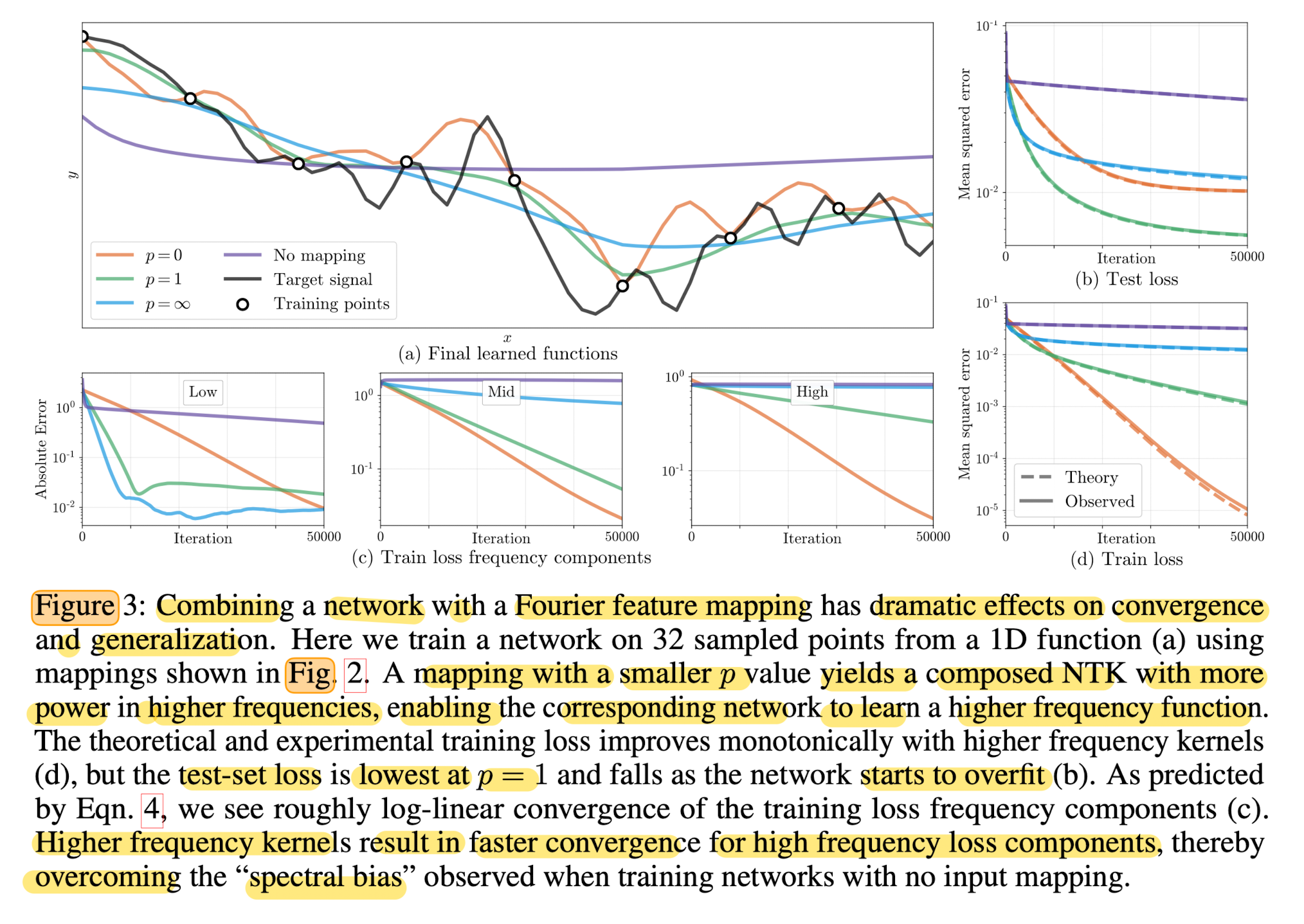
The crucial insight is that applying a fixed mapping $\gamma$ to the input coordinates transforms the network's effective NTK. The new kernel becomes a function of the mapped inputs. When $\gamma$ is the Fourier feature mapping, this new kernel has a much "flatter" spectrum. By explicitly including high-frequency sinusoids in the input, we are effectively boosting the eigenvalues associated with high-frequency functions. This makes the convergence rates for low and high frequencies more comparable, allowing the network to learn fine details efficiently.

Let's start with a high-level overview of this phenomenon.

Now, for a more formal dive into the NTK interpretation. The following reading explains precisely how the Fourier feature mapping reshapes the kernel.

Finally, let's hear this from one of the original authors of the Fourier Features paper.

This is the central mechanism. By pre-processing the input, we change the learning problem into one that is much more suitable for gradient-based optimization of an MLP. The image below, from the Fourier Features paper, shows this in action. The plots in row (c) show that as the frequency of the mapping increases (from "Low" to "High"), the network's training loss on high-frequency components of the signal decreases much faster.

Conclusion

In this lesson, we have dissected the simple yet profound solution to the spectral bias problem that plagued early attempts at implicit neural representations. By mapping low-dimensional input coordinates into a higher-dimensional feature space using a bank of sinusoids, we fundamentally change the network's learning dynamics.

Key Takeaways:

• Positional Encoding as Feature Engineering: Positional encoding is a pre-processing step that creates a rich set of features by applying sine and cosine functions of varying frequencies to the input coordinates.
• Multi-Scale Input: This provides the network with features that are sensitive to changes in the input at many different scales, allowing it to learn both coarse, low-frequency structures and fine, high-frequency details.
• Overcoming Spectral Bias via NTK: From a theoretical standpoint, this input mapping transforms the MLP's effective Neural Tangent Kernel. It "flattens" the kernel's spectrum, increasing the eigenvalues associated with high-frequency functions and thus dramatically speeding up their convergence during training.
• The Key to NeRF: This technique is the critical architectural innovation that allows the NeRF MLP to represent the complex, high-frequency color and density fields necessary for photorealistic view synthesis.

Preview of the Next Lesson:

We now understand the two core components of the NeRF representation: an MLP that acts as a universal function approximator, and positional encoding that enables it to learn high-frequency detail. But a representation is useless if you can't generate an image from it. In the next lesson, we will shift our focus from representation to rendering. We will derive the classical volumetric rendering equation, the mathematical formula used to synthesize the color of a single pixel by accumulating color and density samples along a camera ray.