Understanding the Full NeRF Architecture

Recommended resources

The freely available resources this lesson will direct you to.

Welcome back. In our previous lessons, we assembled two of the three main pillars required for NeRF. First, we saw how to use positional encoding to enable a simple MLP to represent high-frequency 3D scene details. Second, we derived the volume rendering equation, the mathematical tool that transforms a set of color and density samples along a ray into a single pixel color.

Now, we will put everything together. This lesson details the complete NeRF architecture, revealing how the MLP and the rendering equation are integrated into a cohesive system. We will dissect the design of the core network and, most importantly, explore hierarchical volume sampling—a clever, two-stage optimization that is critical to NeRF's ability to render sharp, detailed scenes efficiently.

By the end of this lesson, you will have a full blueprint of the NeRF model, from the 5D coordinate input to the final rendered pixel, preparing you to tackle the implementation in our upcoming sessions.

The Full NeRF Pipeline: A Bird's-Eye View

Let's start with a high-level diagram of the entire process. This will serve as our roadmap for the lesson.

A high-level schematic of the NeRF architecture. This diagram shows the flow from the 5D input, through positional encoding and the MLP, to the final rendering via a two-pass coarse and fine sampling strategy.

As the diagram illustrates, the process involves several key stages:

A 5D input $(x, d)$ is positionally encoded.
The encoded input is passed through an MLP to predict density $σ$ and color $c$ .
A "coarse" model is used to perform an initial, rough sampling along the ray.
The results of the coarse pass are used to inform a more targeted, "fine" sampling.
The final color is rendered using the results from the fine pass.

Let's break down each of these components in detail.

The Core MLP: An Asymmetric Design

The heart of NeRF is a standard Multi-Layer Perceptron (MLP). While it's a simple feedforward network, its internal design has a crucial asymmetry that reflects the physics of light. The goal is to predict volume density $σ$ , which determines the geometry of the scene, and the RGB color $c$ , which determines its appearance.

Here's a concise overview of the architecture from one of the NeRF authors, Jon Barron.

Jon Barron - Understanding and Extending Neural Radiance Fields

This video clip explains the basic structure of the MLP used in NeRF.

Watch the section from the MLP architecture. Notice how the input is a 5D coordinate and the output is color and density.

The key insight is that the shape of an object shouldn't change depending on your viewing angle, but its appearance (e.g., reflections) should. NeRF's architecture is designed to enforce this physical constraint.

Let's examine the specifics of this design.

The Annotated NeRF – Training on Custom Dataset ...

This article provides a clear diagram and explanation of the MLP's structure.

Read the section NeRF MLP Network and review the detailed diagram in the section NeRF Model Architecture. Focus on how the position \mathbf{x} and viewing direction \mathbf{d} are processed differently.

The architecture can be summarized as follows:

Input: The positionally encoded 3D location $γ (x)$ is fed into the network.
Position Processing: The input passes through a series of 8 fully-connected layers (typically 256 channels wide) with ReLU activations. A skip connection concatenates the input again at the 5th layer, which helps with training deeper networks.
Density Prediction: The output of the 8th layer is passed to a single linear layer to produce the volume density $σ$ . Notice that $σ$ is a function of position $x$ only.
Direction Processing: The feature vector from the 8th layer is then concatenated with the positionally encoded 2D viewing direction $γ (d)$ .
Color Prediction: This combined vector is passed through one final linear layer (typically 128 channels wide) and then a sigmoid activation to produce the final view-dependent RGB color $c$ .

Socratic Question: Why is the volume density $σ$ predicted based only on the 3D position $x$ , while the color $c$ depends on both position $x$ and viewing direction $d$ ? What physical properties does this architectural choice allow the model to learn?

Answer

This design choice enforces a strong physical prior. The volume density $\sigma$ represents the "substance" or geometry of the scene. The geometry of an object is intrinsic to its location in space and should not change depending on where you view it from. By making $\sigma$ dependent only on $\mathbf{x}$, the network is forced to learn a consistent, view-independent geometry.

Conversely, the color $c$ is made dependent on both $x$ and $d$ . This allows the network to model non-Lambertian, or view-dependent, effects. This is how NeRF can capture phenomena like specular highlights—the bright glints of light you see on shiny surfaces—which appear only when the viewing angle is aligned correctly with the light source and the surface normal. Jon Barron's video explains this beautifully with a visualization of a boat's reflection.

The Problem with Naive Sampling

Now that we have our MLP, the most straightforward approach to rendering would be:

Cast a ray for a pixel.
Divide the ray into $N$ uniform intervals.
Pick one random sample from each interval (this is called stratified sampling).
Query the MLP for $(c_{i}, σ_{i})$ at each sample point.
Use the discrete volume rendering equation to compute the pixel color.

This process is simple and differentiable, but it's highly inefficient.

Socratic Question: Imagine a scene with a small object floating in a large, empty room. If we cast a ray that passes mostly through empty space before hitting the object, where are the majority of our $N$ samples "wasted"?

Answer

The samples are wasted in the empty space. In these regions, the volume density $\sigma$ will be close to zero. According to the volume rendering equation, the weight for each sample, $w_i = T_i (1 - \exp(-\sigma_i \delta_i))$, will also be near zero. This means these samples contribute almost nothing to the final pixel color, yet we expend computational resources querying the network for them. We are essentially sampling blindly, without regard to where the actual content of the scene is located.

The Solution: Hierarchical Volume Sampling

To address this inefficiency, NeRF employs a more intelligent, two-pass strategy called hierarchical volume sampling. The core idea is to use a "coarse" pass to identify regions of interest along the ray and then focus a "fine" pass on sampling those regions more densely.

This involves training two networks simultaneously: a coarse network ( $F_{θ}^{c}$ ) and a fine network ( $F_{θ}^{f}$ ). They share the same architecture but have independent sets of weights.

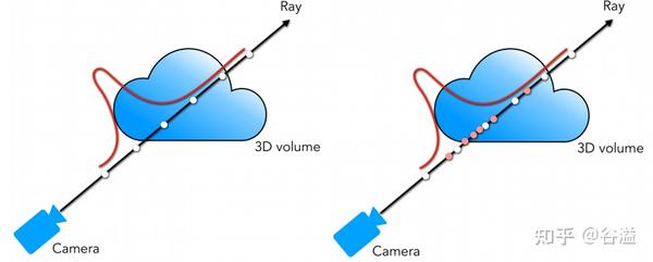
Illustration of hierarchical sampling. (Left) A coarse pass with uniformly spaced samples (white dots). The red curve indicates the density distribution learned by the coarse network. (Right) A fine pass samples more densely (pink dots) in the regions where the coarse network found high density.

Step 1: The Coarse Pass

First, we sample a set of $N_{c}$ locations along the ray using stratified sampling, just like in the naive approach. These sample locations $z_{c} = {z_{1}, z_{2}, \dots, z_{N_{c}}}$ are fed into the coarse network $F_{θ}^{c}$ . We then perform volume rendering using the output from this network to get a set of weights $w_{i}^{c}$ for each sample, as derived in our last lesson:

w_{i}^{c} = T_{i}^{c} (1 - exp (- σ_{i}^{c} δ_{i})) where T_{i}^{c} = exp (- j = 1 \sum i - 1 σ_{j}^{c} δ_{j})

These weights $w_{i}^{c}$ are not just for rendering a preliminary color; they also form a distribution along the ray, indicating where the visible content is likely located.

Step 2: Sampling for the Fine Pass

Next, we treat these weights as the basis for importance sampling. We normalize them to form a piecewise-constant probability density function (PDF) along the ray:

p^(z_{i}) = \frac{w _{i}^{c}}{\sum _{j = 1}^{N_{c}} w _{j}^{c}}

Now, we sample a second set of $N_{f}$ locations, $z_{f}$ , by drawing from this distribution. This is done using a technique called inverse transform sampling. We can understand this process intuitively:

Compute the cumulative distribution function (CDF) from the PDF $p^(z_{i})$ .
Draw $N_{f}$ uniform random numbers between 0 and 1.
For each uniform random number, find the corresponding sample location $z$ on the CDF. This "inverts" the CDF.

This procedure effectively concentrates our new samples in regions that the coarse network identified as important (i.e., having high weights).

The following resource provides an exceptionally clear, code-level explanation of how this is implemented.

NeRF: A Volume Rendering Perspective

This section of Yue Yu's blog post dives into the sample_pdf function from the PyTorch implementation of NeRF, which performs inverse transform sampling.

Read the section on Hierarchical sampling. Focus on understanding the logic: How the weights from the coarse pass are converted into a PDF, and then a CDF. How uniform samples u are used with torch.searchsorted to find the correct "bins" to sample from. How the final sample locations are determined by linear interpolation within these bins.

Step 3: The Fine Pass and Final Render

Finally, we combine our two sets of samples—the initial $N_{c}$ stratified samples and the $N_{f}$ importance samples—to form a total set of $N_{c} + N_{f}$ points. All of these points are then passed to the fine network $F_{θ}^{f}$ . The output from this fine network is used to compute the final, high-quality pixel color $C^_{f} (r)$ using the same volume rendering equation.

The Combined Loss Function

During training, both the coarse and fine renders are compared to the ground truth pixel color $C (r)$ . The total loss is the sum of the mean squared error for both networks:

L = r \in R \sum (∥ C^_{c} (r) - C (r) ∥_{2}^{2} + ∥ C^_{f} (r) - C (r) ∥_{2}^{2})

where $R$ is the batch of rays being trained on.

While $C^_{f}$ is the final output we care about, including $C^_{c}$ in the loss acts as a powerful form of regularization. It forces the coarse network to produce a meaningful, non-trivial prediction, which in turn provides a much better proposal distribution for the fine network's sampling stage. This makes the entire training process more stable and effective.

Conclusion

We have now assembled the full NeRF architecture. It is an elegant system that combines a simple MLP with classical computer graphics principles and a clever sampling strategy.

Key Takeaways:

Core MLP Architecture: NeRF uses a simple MLP with an asymmetric design. Volume density $σ$ is a function of position $x$ only, enforcing view-independent geometry. Color $c$ is a function of both position $x$ and viewing direction $d$ , allowing the model to capture view-dependent effects like specularity.
Hierarchical Volume Sampling: This two-pass system is NeRF's key optimization.
- A coarse network uses stratified sampling to create a rough render and a proposal distribution (the weights $w_{i}^{c}$ ).
- This distribution is used to perform importance sampling, generating a second set of samples concentrated in relevant regions of the scene.
- A fine network uses the combined set of samples to produce the final, high-quality render.
Combined Loss: The training loss includes the error from both the coarse and fine networks. This regularizes the coarse network, forcing it to provide a useful proposal for the fine sampling stage.

Preview of the Next Lesson:

With the complete architectural blueprint in hand, we are ready to begin implementation. In our next lessons, we will start writing the code for the core components of NeRF. We will begin by implementing the crucial positional encoding function from scratch, followed by the differentiable volume renderer itself, turning the equations we've learned into functional Python code.