Positional Encoding for 3D Coordinates & Viewing Directions in Python

Welcome back. In our previous lesson, we assembled the complete architectural blueprint for NeRF, from the asymmetric MLP design to the efficient two-pass hierarchical volume sampling strategy. You now have a high-level understanding of how all the components fit together to turn 5D coordinates into beautifully rendered images.

With that blueprint in hand, our focus now shifts from theory to practice. We will begin the exciting process of implementing a NeRF model from scratch. As with any complex system, we will build it piece by piece, ensuring we understand the role and implementation of each component. We'll start with the very first block in the NeRF pipeline: positional encoding. This lesson will guide you through translating the mathematical concept of Fourier feature mapping, which we've discussed as the solution to spectral bias, into a functional Python implementation.

The Problem Revisited: Spectral Bias

Before we write any code, let's briefly revisit why positional encoding is not just a minor trick, but an absolutely essential component for NeRF. As we've discussed, standard multi-layer perceptrons (MLPs) have an inherent weakness known as spectral bias. They are naturally biased towards learning low-frequency functions and struggle to represent the kind of high-frequency detail found in natural images and 3D scenes, such as sharp edges, fine textures, and intricate geometry.

Feeding raw (x, y, z) coordinates directly to an MLP results in blurry, over-smoothed outputs, even if the network has more than enough capacity to memorize the scene. The following video provides a powerful visual demonstration of this exact problem and introduces the solution.

The "Fourier feature mapping" mentioned in the video is exactly what the NeRF paper calls positional encoding. By mapping the low-dimensional input coordinates into a higher-dimensional space using a series of sine and cosine functions, we make it dramatically easier for the network to learn high-frequency variations.

The Mechanism of Positional Encoding

The core idea is to take a single scalar value $p$ (which could be an x, y, or z coordinate) and transform it using a set of sinusoids with exponentially increasing frequencies. The encoding function $\gamma (\cdot )$ is defined as:

Let's break this down:

• $p$: A single scalar input coordinate.
• $L$: A hyperparameter that defines how many frequency bands we use. In NeRF, this is set to 10 for positions and 4 for viewing directions.
• Frequencies: The sequence of frequencies is $2^0,2^1,2^2,\dots ,2^{L-1}$.
• Output: For each frequency, we compute a sin and cos value. The final encoding for the single scalar $p$ is a vector of length $2L$.

When we apply this to a 3D coordinate $\mathbf{x}=(x,y,z)$, we compute $\gamma (x)$, $\gamma (y)$, and $\gamma (z)$ independently and concatenate the results. Thus, a 3D vector is mapped to a vector of length $3\times 2L$.

The following image provides a great visual intuition for this process. The XY-coordinates on the left are mapped into a set of feature maps on the right, each corresponding to a different frequency sinusoid.

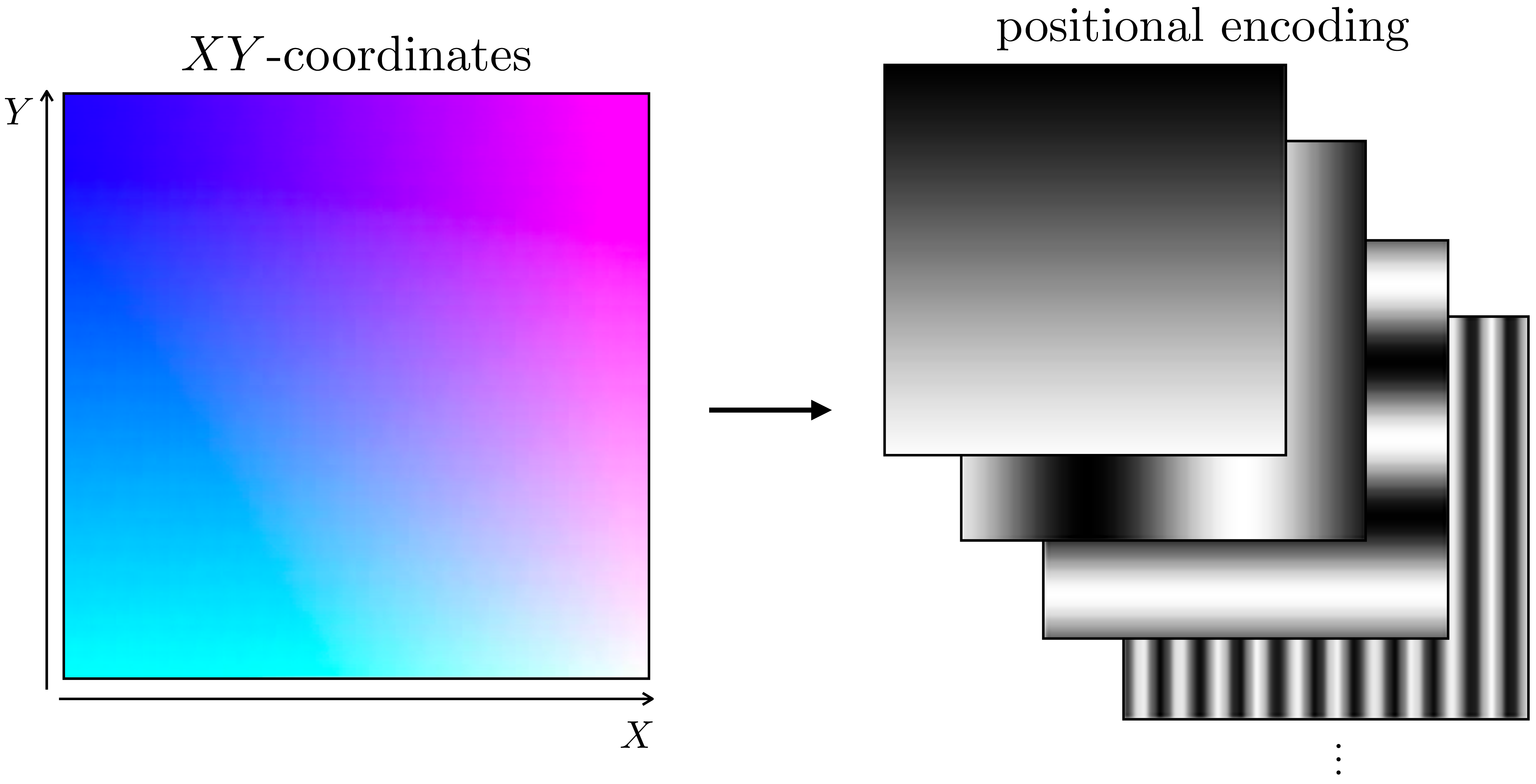
An XY-coordinate plane (left) is transformed by positional encoding into a stack of feature maps (right). Each map represents a sine or cosine function at a different spatial frequency, giving the network access to information at multiple scales.

To build a deeper intuition for how this helps the network, the following video explains that these different frequencies give the network the ability to focus on details at different scales.

From Formula to Python Code

Now, let's translate the formula for $\gamma (p)$ into a Python function using PyTorch. Our goal is to create a function that takes a batch of coordinates (e.g., a tensor of shape (N, 3)) and returns the high-dimensional encoding.

Before looking at a complete implementation, take a moment to think through the logic.

Socratic Question: Suppose you have an input tensor x of shape (N, 3) representing N 3D points. How would you structure the computation in a vectorized way using PyTorch? Specifically, how can you combine x with a 1D tensor of frequencies [1, 2, 4, ...] to efficiently compute all the sin and cos values without a nested loop over each point and each coordinate?

Now, let's examine a clear and direct implementation. The following resource provides a positional_encoding function that uses a simple loop, which makes the connection to the formula very explicit.

Implementing and Testing the Function

Based on the implementation from the resource you just read, we can create our own function and test it. The code below defines positional_encoding and then applies it to mock tensors representing spatial coordinates and viewing directions, using the same hyperparameters (L=10 for position, L=4 for direction) as the original NeRF paper.

import torch

def positional_encoding(x, num_frequencies):
    """
    Applies positional encoding to a tensor of coordinates.

    Args:
        x (torch.Tensor): Input tensor of shape (N, D), where N is the number of points
                          and D is the dimension of each point (e.g., 3 for 3D coordinates).
        num_frequencies (int): The number of frequencies (L) to use for the encoding.

    Returns:
        torch.Tensor: The encoded tensor of shape (N, D * 2 * num_frequencies).
    """
    # Initialize a list to hold the encoded components.
    # We will start with the original input, though many implementations omit this.
    # The original NeRF paper's formula does not include the raw input, so we'll stick to that.
    encoding_list = []

    # Generate the frequency bands: [2^0, 2^1, ..., 2^(L-1)]
    frequencies = 2. ** torch.arange(num_frequencies)

    # Loop through each frequency
    for freq in frequencies:
        # For each frequency, apply sin and cos to the scaled input
        encoding_list.append(torch.sin(freq * x))
        encoding_list.append(torch.cos(freq * x))

    # Concatenate all components along the last dimension
    # The result is a tensor where for each point, you have:
    # [sin(f1*x), cos(f1*x), sin(f2*x), cos(f2*x), ...]
    return torch.cat(encoding_list, dim=-1)

# --- DEMONSTRATION ---

# Define hyperparameters from the NeRF paper
L_pos = 10  # Number of frequencies for position
L_dir = 4   # Number of frequencies for direction
batch_size = 8192  # An example number of rays/points

# 1. Encode 3D spatial coordinates (x, y, z)
# Create a dummy batch of 3D coordinates
coords = torch.randn(batch_size, 3)
encoded_coords = positional_encoding(coords, num_frequencies=L_pos)

print("--- Spatial Coordinates ---")
print(f"Original coords shape: {coords.shape}")
# Expected output dimension: 3 (dims) * 2 (sin/cos) * 10 (freqs) = 60
print(f"Encoded coords shape:  {encoded_coords.shape}")
print("-" * 25)


# 2. Encode 3D viewing directions (d)
# Create a dummy batch of 3D directions and normalize them to be unit vectors
view_dirs = torch.randn(batch_size, 3)
view_dirs = view_dirs / torch.linalg.norm(view_dirs, dim=-1, keepdim=True)
encoded_dirs = positional_encoding(view_dirs, num_frequencies=L_dir)

print("--- Viewing Directions ---")
print(f"Original view dirs shape: {view_dirs.shape}")
# Expected output dimension: 3 (dims) * 2 (sin/cos) * 4 (freqs) = 24
print(f"Encoded view dirs shape:  {encoded_dirs.shape}")
print("-" * 25)

Running this script demonstrates that our function correctly transforms the low-dimensional inputs into the high-dimensional feature vectors required by the NeRF MLP.

Socratic Question: The NeRF authors chose $L=10$ for position and $L=4$ for direction. Why use fewer frequencies for the viewing direction? What does this choice imply about the function the network is expected to learn for view-dependent effects versus geometric structure?

Conclusion

In this lesson, we have taken our first concrete step in building a Neural Radiance Field. We translated the mathematical formulation of positional encoding into a working Python function and verified its behavior.

Key Takeaways:

• Spectral Bias: MLPs are inherently poor at learning high-frequency functions, a problem that positional encoding directly solves.
• Fourier Feature Mapping: Positional encoding maps low-dimensional coordinates to a higher-dimensional feature space using a set of sine and cosine functions at exponentially increasing frequencies.
• Implementation: The encoding function can be implemented straightforwardly in PyTorch by looping through frequency bands and concatenating the sin and cos results.
• NeRF-specifics: In NeRF, positional encoding is applied separately to the 3D positions ($L=10$) and 3D viewing directions ($L=4$), creating input vectors of dimension 60 and 24, respectively.

Preview of the Next Lesson:

With our input encoding function complete, we are now ready to tackle the next major component of the NeRF pipeline: the volume rendering itself. In the next lesson, we will derive and implement the differentiable volume rendering equation. This is the function that takes the $\sigma$ (density) and $\mathbf{c}$ (color) outputs from the MLP for a set of points along a ray and composites them into a single, final pixel color.